There’s a fascinating dichotomy in artificial intelligence between statistics and rules, machine learning and expert systems. Newcomers to artificial intelligence (AI) regard machine learning as innately superior to brittle rules-based systems, while the history of this field reveals both rules and probabilistic learning are integral components of AI.
This fact is perhaps nowhere truer than in establishing explainable AI, which is central to the long-term business value of AI front-office use cases.
Granted, simple machine learning can automate backend processes. However, the full extent of deep learning or complex neural networks — which are much more accurate than basic machine learning — for mission-critical decision-making and action requires explainability.
Using rules (and rules-based systems) to explicate machine learning results creates explainable AI. Many of the far-reaching applications of AI at the enterprise level — deploying it to combat financial crimes, to predict an individual’s immediate and long-term future in health care, for example — require explainable AI that’s fair, transparent and regulatory compliant.
Rules can explain machine learning results for these purposes and others.
AllegroGraph provides two ways to add metadata to triples. The first one is very similar to what typical property graph databases provide: we use the named graph of triples to store meta data about that triple. The second approach is what we have termed triple attributes. An attribute is a key/value pair associated with an individual triple. Each triple can have any number of attributes. This approach, which is built into AllegroGraph’s storage layer, is especially handy for security and bookkeeping purposes. Most of this article will discuss triple attributes but first we quickly discuss the named graph (i.e. fourth element or quad) approach.
1.0 The Named Graph for Properties
Semantic Graph Databases are actually defined by the W3C standard to store RDF as ‘Quads’ (Named Graph, Subject, Predicate, and Object). The ‘Triple Store’ terminology has stuck even though the industry has moved on to storing quads. We believe using the named graph approach to store metadata about triples is richer model that the property graph database method.
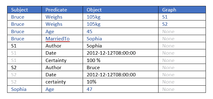
The best way to understand this is to give an example. Below we see two statements about Bruce weighing 105 kilos. The triple portions (subject, predicate, object) are identical but the named graphs (fourth elements) differ. They are used to provide additional information about the triples. The graph values are S1 and S2. By looking at these graphs we see that
The author of the first triple (with graph S1) is Sophia and the author of the second (with graph S2) is Bruce (who is also the subject of the two triples).
Sophia is 100% certain about her statement while Bruce is only 10% certain about his.
Using the named graph we can do even more than a property graph database, as the value of a graph can itself be a node, and is the subject of various triples which specify the original triple’s author, date, and certainty. Additional triples tell us the ages of the authors and the fact that the authors are married.
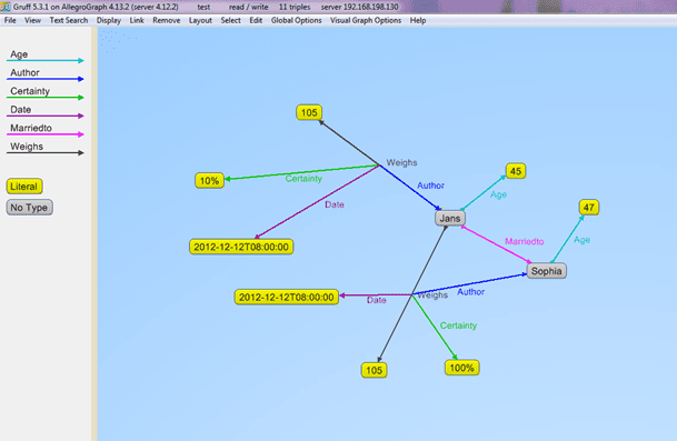
Here is the data displayed in Gruff, AllegroGraph’s associated triple store browser:
Using named graphs for a triple’s metadata is a powerful tool but it does have limitations: (1) only one graph value can be associated with a triple, (2) it can be important that metadata is stored directly and physically with the triple (with named graphs, the actual metadata is usually stored in additional triples with the graph as the subject, as in the example above), and (3) named graphs have competing uses and may not be available for metadata.
2.0 The Triple Attributes approach
AllegroGraph uniquely offers a mechanism called triple attributes where a collection of user defined key/value pairs can be stored with each individual triple. The advantage of this approach is manyfold, but the original use case was designed for triple level security for an Intelligence agency.
By having triple attributes physically connected to the triples in the storage layer we can provide a very powerful and flexible mechanism to protect triples at the lowest possible level in AllegroGraph’s architecture. Our first example below shows this use case in great detail. Other use cases are for example to add weights or costs to triples, to be used in graph algorithms. Or we can add a recorded time or expiration times to a triple and use that to provide a time machine in AllegroGraph or do automatic clean-up of old data.
This article provides an initial introduction to attributes and the associated concept of static filters, showing how they are set up and used. We start with a security example which also describes the basics of adding attributes to triples and filtering query results based on attribute values. Then we discuss other potential uses of attributes.
2.1 Triple Attribute Basics: a Security Example
One important purpose of attributes, when they were added as a feature, was to allow for very fine triple-level security, so that triples would be visible or invisible to users according to the attributes of the triples and the permissions associated with the query being posed by the user.
Note that users as such do not have attributes. Instead, attribute values are assigned when a query is posed. This is an important point: it is natural to think that there can be an attribute SECURITY-LEVEL, and a triple can have attribute SECURITY-LEVEL=3, and USER1 can have an attribute SECURITY-LEVEL=2 and USER2 can have an attribute SECURITY-LEVEL=4, and the system can require that the user SECURITY-LEVEL attribute must be greater than the triple SECURITY-LEVEL for the triple to be visible to the user. But that is not how attributes work. The triples can have the attribute SECURITY-LEVEL=2 but users do not have attributes. Instead, the filter is made part of the query.
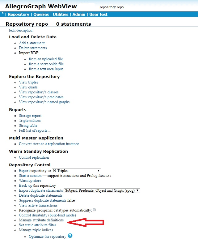
Here is a simple example. We define attributes and static attribute filters using AGWebView. We have a repository named repo. Here is a portion of its AGWebView page:
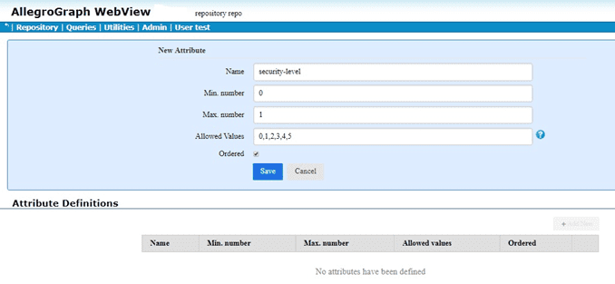
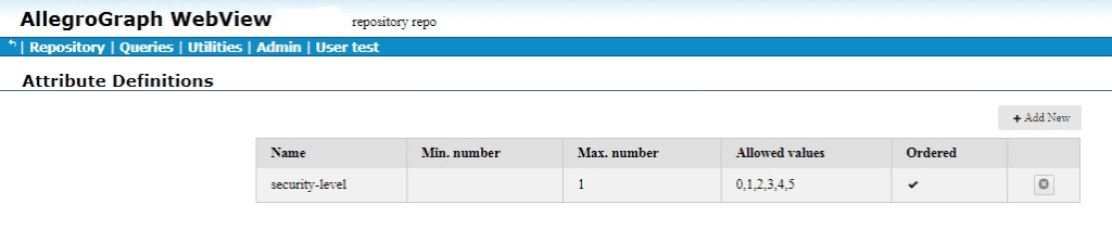
The red arrow points to the commands of interest: Manage attribute definitions and Set static attribute filter. We click on Set static attribute filter to define an attribute. We have filled in the attribute information (name security-level, minimum and maximum number allowed per triple, allowed values, and whether order or not (yes in our case):
We click Save and the attribute is defined:
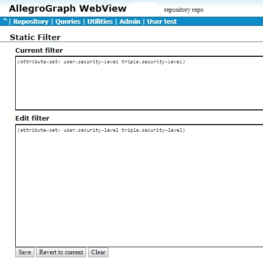
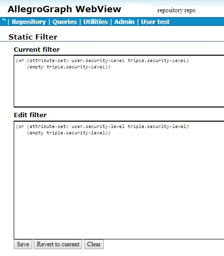
Then we define a filter (on the Set static attribute filter page):
We defined the filter (attribute-set> user.security-level triple.security-level) and clicked Save (the definition appears in both the Edit and the Current fields). The filter says that the “user” security level must be greater than the triple security level. We put “user” in quotes because the user security level is specified as part of the query, and has no direct connection to any specific user.
Here are some triples in a nqx file fr.nqx. The first triple has no attributes and the other three each has a security-level attribute value.
We load this file into a repository which has the security-level attribute defined as above and the static filter mentioned above also defined. (Triples with attributes can also be entered directly when using AGWebView with the Import RDF from a text area input command).
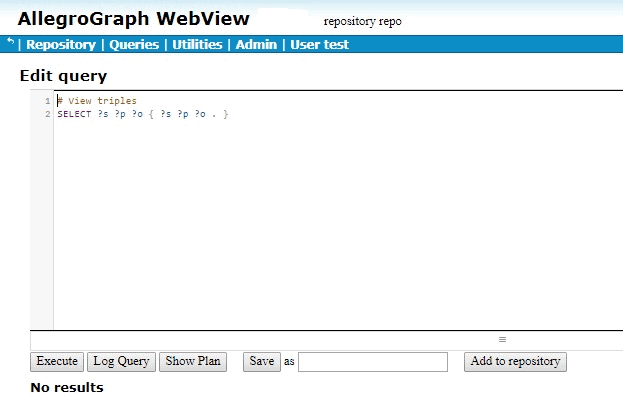
Once the triples are loaded, we click View triples in AGWebView and we see no triples:
This result is often surprising to users just beginning to work with attributes and filters, who may expect the first triple, abbreviated to [emp0 position intern], to be visible, but the system is doing what it is supposed to do. It will only show triples where the security-level of the user posing the query is greater than the security level of the triple. The user has no security level and so the comparison fails, even with triples that have no security-level attribute value. We will describe below how to ensure you can see triples with no attributes.
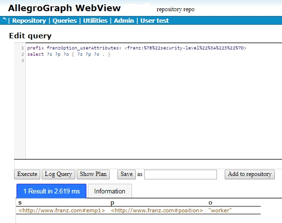
So we need to specify an attribute value to the user posing the query. (As said above, users do not themselves have attribute values. But the attribute value of a user posing a query can be specified as part of the query.) “User” attributes are specified with a prefix like the following:
We will show the results below, but first what are all the % signs and numbers doing there? Why isn’t the prefix just prefix franzOption_userAttributes: <franz:{“security-level”:”3″}>? The issue is that {“security-level”:”3″} won’t read correctly. It must be URL encoded. We do this by going to https://www.urlencoder.org/ (there are other websites that do this as well) and put {“security-level”:”3″} in the first box, click Encode and get %7B%22security-level%22%3A%223%22%7D. We then paste that into the query, as shown above.
When we try that query in AGWebView, we get one result:
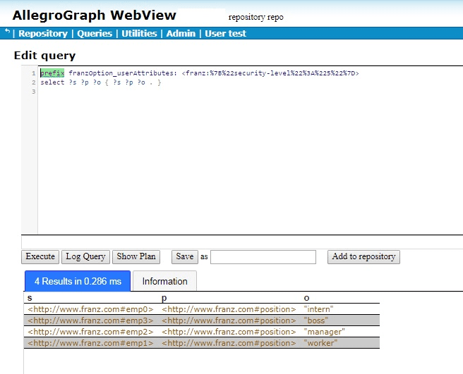
If we encode {“security-level”:”5″} to get the query
emp3 position “boss” emp2 position “manager” emp1 position “worker”
since now the “user” security-level is greater than that of any triples with a security-level attribute. But what about the triple with subject emp0, the triple with no attributes? It does not pass the filter which required that the user attribute be greater than the triple attribute. Since the triple has no attribute value so the comparison failed.
Now a triple will pass the filter if either (1) the “user” security-level is greater than the triple security-level or (2) the triple does not have a security-level attribute. Now the query from above where the user has attribute security-level:”5” will show all the triples with security-level less than 5 and with no attributes at all. That happens to be all four triples so far defined:
The triple
emp0 position “intern”
will now appears as a result in any query where it satisfies the SPARQL select regardless of the security-level of the “user”.
It would be a useful feature that we could associate attributes with actual users. However, this is not as simple as it sounds. Attributes are features of repositories. If I have a REPO1 repository, it can have a bunch of defined attributes and filters but my REPO2 may know nothing about them and its triples may not have any attributes at all, and no attributes are defined, and (as a result) no filters. But users are not repository-linked objects. While a repository can be made read-only or unreadable for a user, users do not have finer repository features. So an interface for providing users with attributes, since it would only make sense on a per-repository basis, requires a complicated interface. That is not yet implemented (though we are considering how it can be done).
Instead, users can have specific prefixes associated with them and that prefix and be included in any query made by the user.
But if all it takes to specify “user” attributes is to put the right line at the top of your SPARQL query, that does not seem to provide much security. There is a feature for users “Allow user attributes via SPARQL PREFIX franzOption_userAttributes” which can restrict a user’s ability to specify “user” attributes in a query, but that is a rather blunt instrument. Instead, the model is that most users (outside of trusted administrators) are not actually allowed to pose SPARQL queries directly. Instead, there is an intermediary program which takes the query a user requests and, having determined the status of the user and what attribute values should be given to the user, modifies the query with the appropriate franzOption_userAttributes prefixes and then sends the query on to the server, following which it captures the results and sends them back to the requesting user. That intermediate program will store the prefix suitable for a user and thus associate “user” attributes with specific users.
2.2 Using attributes as additional data
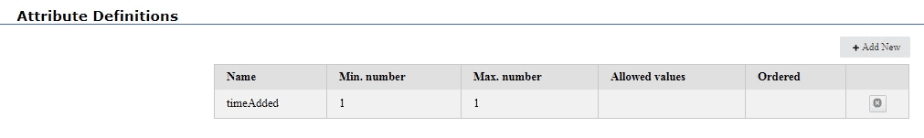
Although triple security is one powerful use of attributes, security is far from the only use. Just as the named graph can serve as additional data, so can attributes. SPARQL queries can use attribute values just as static filters can filter out triples before displaying them. Let us take a simple example: the attribute timeAdded. Every triple we add will have a timeAdded attribute value which will be a string whose contents are a datetime value, such as “2017-09-11T:15:52”. We define the attribute:
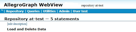
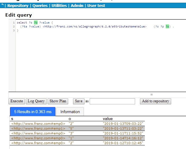
We have a call center with employees making calls. Each call has a ranking from 1 to 5, with 1 the lowest and 5 the highest. We have data on five calls, four from emp0 and one from emp1. Each triples has a timeAdded attribute with a string containing a dateTime value. We load these into a empty repository named at-test where the timeAdded attribute is defined as above:
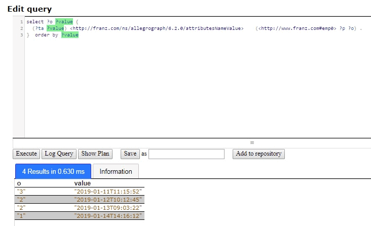
But we are really interested just in emp0 and we would like to see the results ordered by time, that is by the attribute value, so we restrict the query to emp0 as the subject and order the results:
select ?o ?value { (?ta ?value) <http://franz.com/ns/allegrograph/6.2.0/attributesNameValue> (<http://www.franz.com#emp0> ?p ?o) . } order by ?value
There are the results for emp0, who is clearly having difficulties because the call rankings have been steadily falling over time.
Another example using timeAdded is employee salary data. In the Human Resources data, the salary of an employee is stored:
emp0 hasSalary 50000
Now emp0 gets a raise to 55000. So we delete the triple above and add the triple
emp0 hasSalary 55000
But that is not satisfactory because we have lost the salary history. If the boss asks “How much was emp0 paid initially?” we cannot answer. There are various solutions. We could define a salary change object, with predicates effectiveDate, previousSalary, newSalary, and so on:
and that would work fine, but perhaps it is more setup and effort than is needed. Suppose we just have hasSalary triples each with a timeAdded attribute. Then the current salary is the latest one and the history is the ordered list. Here that idea is worked out:
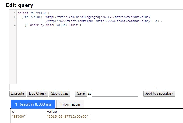
What is the current salary? A simple SPARQL query tells us:
select ?o ?value { (?ta ?value) <http://franz.com/ns/allegrograph/6.2.0/attributesNameValue> (<http://www.franz.com#emp0> <http://www.franz.com#hasSalary> ?o) . } order by desc(?value) limit 1
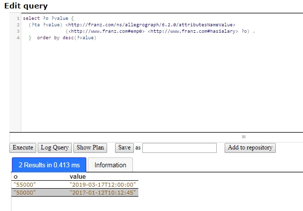
The salary history is provided by the same query without the LIMIT:
select ?o ?value { (?ta ?value) <http://franz.com/ns/allegrograph/6.2.0/attributesNameValue> (<http://www.franz.com#emp0> <http://www.franz.com#hasSalary> ?o) . } order by desc(?value)
This method of storing salary data may not easily support more complex questions which might be easily answered if we went the salaryChange object route mentioned above but if you are not looking to ask those questions, you should not do the extra work (and the risk of data errors) required.
You could use the graph of each triple for the timeAdded. All the examples above would work with minor tweaks. But there are many uses for the named graph of a triple. Attributes are available and using them for one purpose does not restrict their use for other purposes.
There are many reasons for working with JSON-LD. The major search engines such as Google require ecommerce companies to mark up their websites with a systematic description of their products and more and more companies use it as an easy serialization format to share data.
The benefit for your organization is that you can now combine your documents with graphs, graph search and graph algorithms. Normally when you store documents in a document store you set up your documents in such a way that it is optimized for direct retrieval queries. Doing complex joins for multiple types of documents or even doing a shortest path through a mass of object (types) is however very complicated. Storing JSON-LD objects in AllegroGraph gives you all the benefits of a document store and you can semantically link objects together, do complex joins and even graph search.
A second benefit is that, as an application developer, you do not have to learn the entire semantic technology stack, especially the part where developers have to create individual triples or edges. You can work with the JSON data serialization format that application developers usually prefer.
In the following you will first learn about JSON-LD as a syntax for semantic graphs. After that we will talk more about using JSON-LD with AllegroGraph as a document-graph-store.
Setup
You can use Python 2.6+ or Python 3.3+. There are small setup differences which are noted. You do need agraph-python-101.0.1 or later.
Mimicking instructions in the Installation document, you should set up the virtualenv environment.
Create an environment named jsonld:
python3-mvenvjsonld
or
python2-mvirtualenvjsonld
Activate it:
Using the Bash shell:
sourcejsonld/bin/activate
Using the C shell:
sourcejsonld/bin/activate.csh
Install agraph-python:
pipinstallagraph-python
And start python:
python
[various startup and copyright messages]
>>>
We assume you have an AllegroGraph 6.5.0 server running. We call ag_connect. Modify the host, port, user, and password in your call to their correct values:
from franz.openrdf.connect import ag_connect
with ag_connect('repo', host='localhost', port='10035',
                user='test', password='xyzzy') as conn:
    print (conn.size())
If the script runs successfully a new repository named repo will be created.
JSON-LD setup
We next define some utility functions which are somewhat different from what we have used before in order to work better with JSON-LD. createdb() creates and opens a new repository and opendb() opens an existing repo (modify the values of host, port, user, and password arguments in the definitions if necessary). Both return repository connections which can be used to perform repository operations. showtriples() displays triples in a repository.
importosimportjson,requests,copyfromfranz.openrdf.sail.allegrographserverimportAllegroGraphServerfromfranz.openrdf.connectimportag_connectfromfranz.openrdf.vocabulary.xmlschemaimportXMLSchemafromfranz.openrdf.rio.rdfformatimportRDFFormat# Functions to create/open a repo and return a RepositoryConnection# Modify the values of HOST, PORT, USER, and PASSWORD if necessarydefcreatedb(name):returnag_connect(name,host="localhost",port=10035,user="test",password="xyzzy",create=True,clear=True)defopendb(name):returnag_connect(name,host="localhost",port=10035,user="test",password="xyzzy",create=False)defshowtriples(limit=100):statements=conn.getStatements(limit=limit)withstatements:forstatementinstatements:print(statement)
Finally we call our createdb function to create a repository and return a RepositoryConnection to it:
conn=createdb('jsonplay')
Some Examples of Using JSON-LD
In the following we try things out with some JSON-LD objects that are defined in json-ld playground: jsonld
The first object we will create is an event dict. Although it is a Python dict, it is also valid JSON notation. (But note that not all Python dictionaries are valid JSON. For example, JSON uses null where Python would use None and there is no magic to automatically handle that.) This object has one key called @context which specifies how to translate keys and values into predicates and objects. The following @context says that every time you see ical: it should be replaced by http://www.w3.org/2002/12/cal/ical#, xsd: by http://www.w3.org/2001/XMLSchema#, and that if you see ical:dtstart as a key than the value should be treated as an xsd:dateTime.
event={"@context":{"ical":"http://www.w3.org/2002/12/cal/ical#","xsd":"http://www.w3.org/2001/XMLSchema#","ical:dtstart":{"@type":"xsd:dateTime"}},"ical:summary":"Lady Gaga Concert","ical:location":"New Orleans Arena, New Orleans, Louisiana, USA","ical:dtstart":"2011-04-09T20:00:00Z"}
Let us try it out (the subjects are blank nodes so you will see different values):
In the above we see that the JSON-LD was correctly translated into triples but there are two immediate problems: first each subject is a blank node, the use of which is problematic when linking across repositories; and second, the object does not have an RDF type. We solve these problems by adding an @id to provide an IRI as the subject and adding a @type for the object (those are at the lines just after the @context definition):
We also create a test function to test our JSON-LD objects. It is more powerful than needed right now (here we just need conn,addData(event) and showTriples() but test will be useful in most later examples. Note the allow_external_references=True argument to addData(). Again, not needed in this example but later examples use external contexts and so this argument is required for those.
Note in the above that we now have a proper subject and a type.
Referencing a External Context Via a URL
The next object we add to AllegroGraph is a person object. This time the @context is not specified as a JSON object but as a link to a context that is stored at http://schema.org/. Also in the definition of the function test above we had this parameter in addData:allow_external_references=True. Requiring that argument explicitly is a security feature. One should use external references only that context at that URL is trusted (as it is in this case).
Adding one person at a time requires doing an interaction with the server for each person. It is much more efficient to add lists of objects all at once rather than one at a time. Note that addData will take a list of dicts and still do the right thing. So let us add a 1000 persons at the same time, each person being a copy of the above person but with a different @id. (The example code is repeated below for ease of copying.)
>>> x = [copy.deepcopy(person) for i in range(1000)]
>>> len(x)
1000
>>> c = 0
>>> for el in x:
    el['@id']= "http://franz.com/person-" + str(c)
    c= c + 1
>>> test(x,maxPrint=10)
(<http://franz.com/person-0>, <http://schema.org/name>, "Jane Doe")
(<http://franz.com/person-0>, <http://schema.org/jobTitle>, "Professor")
(<http://franz.com/person-0>, <http://schema.org/telephone>, "(425) 123-4567")
(<http://franz.com/person-0>, <http://schema.org/url>, <http://www.janedoe.com>)
(<http://franz.com/person-0>, <http://www.w3.org/1999/02/22-rdf-syntax-ns#type>, <http://schema.org/Person>)
(<http://franz.com/person-1>, <http://schema.org/name>, "Jane Doe")
(<http://franz.com/person-1>, <http://schema.org/jobTitle>, "Professor")
(<http://franz.com/person-1>, <http://schema.org/telephone>, "(425) 123-4567")
(<http://franz.com/person-1>, <http://schema.org/url>, <http://www.janedoe.com>)
(<http://franz.com/person-1>, <http://www.w3.org/1999/02/22-rdf-syntax-ns#type>, <http://schema.org/Person>)
>>> conn.size()
5000
>>>
x = [copy.deepcopy(person) for i in range(1000)]
len(x)

c = 0
for el in x:
    el['@id']= "http://franz.com/person-" + str(c)
    c= c + 1

test(x,maxPrint=10)

conn.size()
Adding a Context Directly to an Object
You can download a context directly in Python, modify it and then add it to the object you want to store. As an illustration we load a person context from json-ld.org (actually a fragment of the schema.org context) and insert it in a person object. (We have broken and truncated some output lines for clarity and all the code executed is repeated below for ease of copying.)
context=requests.get("https://json-ld.org/contexts/person.jsonld").json()['@context']# The next produces lots of output, uncomment if desired#contextperson={"@context":context,"@type":"Person","@id":"foaf:person-1","name":"Jane Doe","jobTitle":"Professor","telephone":"(425) 123-4567",}test(person)
Building a Graph of Objects
We start by forcing a key’s value to be stored as a resource. We saw above that we could specify the value of a key to be a date using the xsd:dateTime specification. We now do it again for foaf:birthdate. Then we created several linked objects and show the connections using Gruff.
The following shows the graph that we created in Gruff. Note that this is what JSON-LD is all about: connecting objects together.
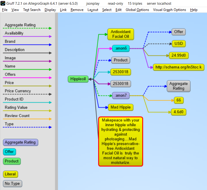
JSON-LD Keyword Directives can be Added at any Level
Here is an example from the wild. The URL https://www.ulta.com/antioxidant-facial-oil?productId=xlsImpprod18731241 goes to a web page advertising a facial oil. (We make no claims or recommendations about this product. We are simply showing how JSON-LD appears in many places.) Look at the source of the page and you’ll find a JSON-LD object similar to the following. Note that @ directives go to any level. We added an @id key.
hippieoil={"@context":"http://schema.org","@type":"Product","@id":"http://franz.com/hippieoil","aggregateRating":{"@type":"AggregateRating","ratingValue":4.6,"reviewCount":73},"description":"""Make peace with your inner hippie while hydrating & protecting against photoaging....Mad Hippie's preservative-free Antioxidant Facial Oil is truly the most natural way to moisturize.""","brand":"Mad Hippie","name":"Antioxidant Facial Oil","image":"https://images.ulta.com/is/image/Ulta/2530018","productID":"2530018","offers":{"@type":"Offer","availability":"http://schema.org/InStock","price":"24.99","priceCurrency":"USD"}}test(hippieoil)
JSON-LD @graphs
One can put one or more JSON-LD objects in an RDF named graph. This means that the fourth element of each triple generated from a JSON-LD object will have the specified graph name. Let’s show in an example.
context={"name":"http://schema.org/name","description":"http://schema.org/description","image":{"@id":"http://schema.org/image","@type":"@id"},"geo":"http://schema.org/geo","latitude":{"@id":"http://schema.org/latitude","@type":"xsd:float"},"longitude":{"@id":"http://schema.org/longitude","@type":"xsd:float"},"xsd":"http://www.w3.org/2001/XMLSchema#"}place={"@context":context,"@id":"http://franz.com/place1","@graph":{"@id":"http://franz.com/place1","@type":"http://franz.com/Place","name":"The Empire State Building","description":"The Empire State Building is a 102-story landmark in New York City.","image":"http://www.civil.usherbrooke.ca/cours/gci215a/empire-state-building.jpg","geo":{"latitude":"40.75","longitude":"73.98"}}}
and here is the result:
>>> test(place, maxPrint=3)
(<http://franz.com/place1>, <http://schema.org/name>, "The Empire State Building", <http://franz.com/place1>)
(<http://franz.com/place1>, <http://schema.org/description>, "The Empire State Building is a 102-story landmark in New York City.", <http://franz.com/place1>)
(<http://franz.com/place1>, <http://schema.org/image>, <http://www.civil.usherbrooke.ca/cours/gci215a/empire-state-building.jpg>, <http://franz.com/place1>)
>>>
Note that the fourth element (graph) of each of the triples is <http://franz.com/place1>. If you don’t add the @id the triples will be put in the default graph.
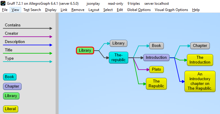
Here a slightly more complex example:
library={"@context":{"dc":"http://purl.org/dc/elements/1.1/","ex":"http://example.org/vocab#","xsd":"http://www.w3.org/2001/XMLSchema#","ex:contains":{"@type":"@id"}},"@id":"http://franz.com/mygraph1","@graph":[{"@id":"http://example.org/library","@type":"ex:Library","ex:contains":"http://example.org/library/the-republic"},{"@id":"http://example.org/library/the-republic","@type":"ex:Book","dc:creator":"Plato","dc:title":"The Republic","ex:contains":"http://example.org/library/the-republic#introduction"},{"@id":"http://example.org/library/the-republic#introduction","@type":"ex:Chapter","dc:description":"An introductory chapter on The Republic.","dc:title":"The Introduction"}]}
So far we have treated JSON-LD as a syntax to create triples. Now let us look at the way we can start using AllegroGraph as a combination of a document store and graph database at the same time. And also keep in mind that we want to do it in such a way that you as a Python developer can add documents such as dictionaries and also retrieve values or documents as dictionaries.
Setup
The Pythonsourcefilejsonld_tutorial_helper.py contains various definitions useful for the remainder of this example. Once it is downloaded, do the following (after adding the path to the filename):
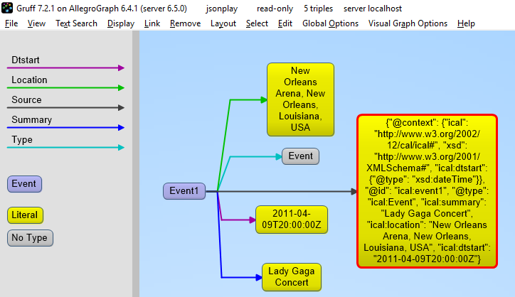
Let’s use our event structure again and see how we can store this JSON document in the store as a document. Note that the addData call includes the keyword: json_ld_store_source=True.
event={"@context":{"@id":"ical:event1","@type":"ical:Event","ical":"http://www.w3.org/2002/12/cal/ical#","xsd":"http://www.w3.org/2001/XMLSchema#","ical:dtstart":{"@type":"xsd:dateTime"}},"ical:summary":"Lady Gaga Concert","ical:location":"New Orleans Arena, New Orleans, Louisiana, USA","ical:dtstart":"2011-04-09T20:00:00Z"}
The jsonld_tutorial_helper.py file defines the function store as simple wrapper around addDatathat always saves the JSON source. For experimentation reasons it also has a parameter fresh to clear out the repository first.
>>> store(conn,event, fresh=True)
If we look at the triples in Gruff we see that the JSON source is stored as well, on the root (top-level @id) of the JSON object.
For the following part of the tutorial we want a little bit more data in our repository so please look at the helper file jsonld_tutorial_helper.py where you will see that at the end we have a dictionary named obs with about 9 diverse objects, mostly borrowed from the json-ld.org site: a person, an event, a place, a recipe, a group of persons, a product, and our hippieoil.
First let us store all the objects in a fresh repository. Then we check the size of the repo. Finally, we create a freetext index for the JSON sources.
>>> store(conn,[v for k,v in obs.items()], fresh=True)
>>> conn.size()
86
>>> conn.createFreeTextIndex("source",['<http://franz.com/ns/allegrograph/6.4/load-meta#source>'])
>>>
Retrieving values with SPARQL
To simply retrieve values in objects but not the objects themselves, regular SPARQL queries will suffice. But because we want to make sure that Python developers only need to deal with regular Python structures as lists and dictionaries, we created a simple wrapper around SPARQL (see helper file). The name of the wrapper is runSparql.
Here is an example. Let us find all the roots (top-level @ids) of objects and their types. Some objects do not have roots, so None stands for a blank node.
retrieve is another function defined (in jsonld_tutorial_helper.py) for this tutorial. It is a wrapper around SPARQL to help extract objects. Here we see how we can use it. The sole purpose of retrieve is to retrieve the JSON-LD/dictionary based on a SPARQL pattern.
Ok, for a final fun (if you like expensive cars) example: Let us find a thing that is “fast and furious”, that is worth more than $80,000 and that we can pay for in cash:
Gartner Identifies Top 10 Data and Analytics Technology Trends for 2019
According to Donald Feinberg, vice president and distinguished analyst at Gartner, the very challenge created by digital disruption — too much data — has also created an unprecedented opportunity. The vast amount of data, together with increasingly powerful processing capabilities enabled by the cloud, means it is now possible to train and execute algorithms at the large scale necessary to finally realize the full potential of AI.
“The size, complexity, distributed nature of data, speed of action and the continuous intelligence required by digital business means that rigid and centralized architectures and tools break down,” Mr. Feinberg said. “The continued survival of any business will depend upon an agile, data-centric architecture that responds to the constant rate of change.”
Gartner recommends that data and analytics leaders talk with senior business leaders about their critical business priorities and explore how the following top trends can enable them.
Trend No. 5: Graph
Graph analytics is a set of analytic techniques that allows for the exploration of relationships between entities of interest such as organizations, people and transactions.
The application of graph processing and graph DBMSs will grow at 100 percent annually through 2022 to continuously accelerate data preparation and enable more complex and adaptive data science.
Graph data stores can efficiently model, explore and query data with complex interrelationships across data silos, but the need for specialized skills has limited their adoption to date, according to Gartner.
Graph analytics will grow in the next few years due to the need to ask complex questions across complex data, which is not always practical or even possible at scale using SQL queries.
Franz CEO Dr. Jans Aasman Explains how to manage AI Modelling Risks.
AI model risk management has moved to the forefront of contemporary concerns for statistical Artificial Intelligence, perhaps even displacing the notion of ethics in this regard because of the immediate, undesirable repercussions of tenuous machine learning and deep learning models.
AI model risk management requires taking steps to ensure that the models used in artificial applications produce results that are unbiased, equitable, and repeatable.
The objective is to ensure that given the same inputs, they produce the same outputs.
If organizations cannot prove how they got the results of AI risk models, or have results that are discriminatory, they are subject to regulatory scrutiny and penalties.
There’s a growing cry for these standards in other heavily regulated industries such as healthcare, while the burgeoning Fair, Accountable, Transparent movementtypifies the horizontal demand to account for machine learning models’ results.
AI model risk management is particularly critical in finance.
Financial organizations must be able to demonstrate how they derived the offering of any financial product or service for specific customers.
When deploying AI risk models for these purposes, they must ensure they can explain (to customers and regulators) the results that determined those offers.
Although you may not have heard of JavaScript Object Notation Linked Data (JSON-LD), it is already affecting your business. Search engine giant Google has mentioned JSON-LD as a preferred means of adding structured data to webpages to make them considerably easier to parse for more accurate search engine results. The Google use case is indicative of the larger capacity for JSON-LD to increase web traffic for sites and better guide users to the results they want.
Expectations are high for JSON-LD, and with good reason. It effectively delivers the many benefits of JSON, a lightweight data interchange format, into the linked data world. Linked data is the technological approach supporting the World Wide Web and one of the most effective means of sharing data ever devised.
In addition, the growing number of enterprise knowledge graphs fully exploit the potential of JSON-LD as it enables organizations to readily access data stored in document formats and a variety of semi-structured and unstructured data as well. By using this technology to link internal and external data, knowledge graphs exemplify the linked data approach underpinning the growing adoption of JSON-LD — and the demonstrable, recurring business value that linked data consistently provides.
Unraveling the Quandary of Access Layer versus Storage Layer Security
InfoSecurity – February 2019
Dr. Jans Aasman was quoted in this article about how AllegroGraph’s Triple Attributes provide Storage Layer Security.
With horizontal standards such as the General Data Protection Regulation (GDPR) and vertical mandates like the Fair Credit Reporting Act increasing in scope and number, information security is impacted by regulatory compliance more than ever.
Organizations frequently decide between concentrating protection at the access layer via role-based security filtering, or at the storage layer with methods like encryption, masking, and tokenization.
The argument is that the former underpins data governance policy and regulatory compliance by restricting data access according to department or organizational role. However, the latter’s perceived as providing more granular security implemented at the data layer.
A hybrid of access based security and security at the data layer—implemented by triple attributes—can counteract the weakness of each approach with the other’s strength, resulting in information security that Franz CEO Jans Aasman characterized as “fine-grained and flexible enough” for any regulatory requirements or security model.
The security provided by this semantic technology is considerably enhanced by the addition of key-value pairs as JSON objects, which can be arbitrarily assigned to triples within databases. These key-value pairs provide a second security mechanism “embedded in the storage, so you cannot cheat,” Aasman remarked.
When implementing HIPPA standards with triple attributes, “even if you’re a doctor, you can only see a patient record if all your other attributes are okay,” Aasman mentioned.
“We’re talking about a very flexible mechanism where we can add any combination of key-value pairs to any triples, and have a very flexible language to specify how to use that to create flexible security models,” Aasman said.
Semantic Web and Semantic Technology Trends in 2019
Dataversity – January 2019
What to expect of Semantic Web and other Semantic Technologies in 2019? Quite a bit. DATAVERSITY engaged with leaders in the space to get their thoughts on how Semantic Technologies will have an impact on multiple areas.
Dr. Jans Aasman, CEO of Franz Inc. was quoted several times in the article:
Among the semantic-driven AI ventures next year will be those that relate to the healthcare space, says Dr. Jans Aasman, CEO of Semantic Web technology company Franz, Inc:
“In the last two years some of the technologies were starting to get used in production,” he says. “In 2019 we will see a ramp-up of the number of AI applications that will help save lives by providing early warning signs for impending diseases. Some diseases will be predicted years in advance by using genetic patient data to understand future biological issues, like the likelihood of cancerous mutations — and start preventive therapies before the disease takes hold.”
If that’s not enough, how about digital immortality via AI Knowledge Graphs, where an interactive voice system will bring public figures in contact with anyone in the real world? “We’ll see the first examples of Digital Immortality in 2019 in the form of AI Digital Personas for public figures,” says Aasman, whose company is a partner in the Noam Chomsky Knowledge Graph:
“The combination of Artificial Intelligence and Semantic Knowledge Graphs will be used to transform the works of scientists, technologists, politicians, and scholars like Noam Chomsky into an interactive response system that uses the person’s actual voice to answer questions,” he comments.
“AI Digital Personas will dynamically link information from various sources — such as books, research papers, notes and media interviews — and turn the disparate information into a knowledge system that people can interact with digitally.” These AI Digital Personas could also be used while the person is still alive to broaden the accessibility of their expertise.
On the point of the future of graph visualization apps, Aasman notes that:
“Most graph visualization applications show network diagrams in only two dimensions, but it is unnatural to manipulate graphs on a flat computer screen in 2D. Modern R virtual reality will add at least two dimensions to graph visualization, which will create a more natural way to manipulate complex graphs by incorporating more depth and temporal unfolding to understand information within a time perspective.”
2019 Trends In The Internet Of Things: The Makings Of An Intelligent IoT
AI Business – December 2018
2019 will be a crucial year for the Internet of Things for two reasons. Firstly, many of the initial predictions for this application of big data prognosticated a future whereby at the start of the next decade there would be billions of connected devices all simultaneously producing sensor data. The IoT is just a year away from making good on those claims.
Dr. Jans Aasman, Franz’s CEO was quoted by the author:
The IIoT is the evolution of the IoT that will give it meaning and help it actualize the number of connected devices forecast for the start of the next decade. The IIoT will encompass smart cities, edge devices, wearables, deep learning and classic machine learning alongside lesser acknowledged elements of AI in a basic paradigm in which, according to Franz CEO Jans Aasman, “you can look at the past and learn from certain situations what’s likely going to happen. You feed it in your [IoT] system and it does better… then you look at what actually happened and it goes back in your machine learning system. That will be your feedback loop.”
Although deep learning relies on many of the same concepts as traditional machine learning, with “deep learning it’s just that you do it with more computers and more intermediate layers,” Aasman said, which results in higher accuracy levels.
The feedback mechanism described by Aasman has such a tremendous capacity to reform data-driven businesses because of the speed of the iterations provided by low latency IIoT data.
One of the critical learning facets the latter produces involves optimization, such as determining the best way to optimize route deliveries encompassing a host of factors based on dedicated rules about them. “There’s no way in [Hades] that a machine learning system would be able to do the complex scheduling of 6,000 people,” Aasman declared. “That’s a really complicated thing where you have to think of every factor for every person.”
However, constraint systems utilizing multi-step reasoning can regularly complete such tasks and the optimization activities for smart cities. Aasman commented that for smart cities, semantic inferencing systems can incorporate data from traffic patterns and stop lights, weather predictions, the time of year, and data about specific businesses and their customers to devise rules for optimal event scheduling. Once the events actually take place, their results—as determined by KPIs—can be analyzed with machine learning to issue future predictions about how to better those results in what Aasman called “a beautiful feedback loop between a machine learning system and a rules-based system.”
In almost all of the examples discussed above, the IIoT incorporates cognitive computing “so humans can take action for better business results,” Aasman acknowledged. The means by which these advantages are created are practically limitless.
There’s a general consensus throughout the data ecosystem that Data Preparation is the most substantial barrier to capitalizing on data-driven processes. Whether organizations are embarking on Data Science initiatives or simply feeding any assortment of enterprise applications, the cleansing, classifying, mapping, modeling, transforming, and integrating of data is the most time honored (and time consuming) aspect of this process.
 The following is example #19 from our
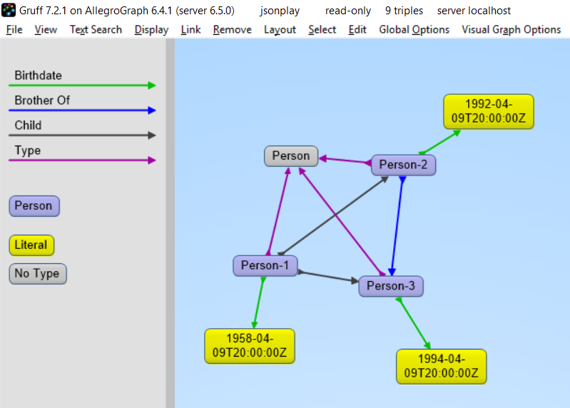
 The objective is to ensure that given the same inputs, they produce the same outputs.