Multi-Master Replication Clusters in Kubernetes and Docker Swarm

For more examples visit – https://github.com/franzinc/agraph-examples

Introduction

In this document we primarily discuss running a Multi-Master Replication cluster (MMR) inside Kubernetes. We will also show a Docker Swarm implementation.

This directory and subdirectories contain code you can use to run an MMR cluster. The second half of this document is entitled Setting up and running MMR under Kubernetes and that is where you’ll see the steps needed to run the MMR cluster in Kubernetes.

MMR replication clusters are different from distributed AllegroGraph clusters in these important ways:

  1. Each member of the cluster needs to be able to make a TCP connection to each other member of the cluster. The connection is to a port computed at run time. The range of port numbers to which a connection is made can be constrained by the agraph.cfg file but typically this will be a large range to ensure that at least one port in that range is not in used.
  2. All members of the cluster hold the complete database (although for brief periods of time they can be out of sync and catching up with one another).

MMR replication clusters don’t quite fit the Kubernetes model in these ways

  1. When the cluster is running normally each instance knows the DNS name or IP address of each other instance. In Kubernetes you don’t want to depend on the IP address of another cluster’s pod as those pods can go away and a replacement started at a different IP address. We’ll describe below our solution to this.
  2. Services are a way to hide the actual location of a pod however they are designed to handle a set of known ports.. In our case we need to connect from one pod to a known-at-runtime port of another pod and this isn’t what services are designed for.
  3. A key feature of Kubernetes is the ability to scale up and down the number of processes in order to handle the load appropriately. Processes are usually single purpose and stateless. An MMR process is a full database server with a complete copy of the repository. Scaling up is not a quick and simple operation – the database must be copied from another node. Thus scaling up is a more deliberate process rather than something automatically done when the load on the system changes during the day.

The Design

  1. We have a headless service for our controlling instance StatefulSet and that causes there to be a DNS entry for the name controlling that points to the current IP address of the node in which the controlling instance runs. Thus we don’t need to hardwire the IP address of the controlling instance (as we do in our AWS load balancer implementation).
  2. The controlling instance uses two PersistentVolumes to store: 1. The repo we’re replicating and 2. The token that other nodes can use to connect to this node. Should the controlling instance AllegroGraph server die (or the pod in which it runs dies) then when the pod is started again it will have access to the data on those two persistent volumes.
  3. We call the other instances in the cluster Copy instances. These are full read-write instances of the repository but we don’t back up their data in a persistent volume. This is because we want to scale up and down the number of Copy instances. When we scale down we don’t want to save the old data since when we scale down we remove that instance from the cluster thus the repo in the cluster can never join the cluster again. We denote the Copy instances by their IP addresses. The Copy instances can find the address of the controlling instance via DNS. The controlling instance will pass the cluster configuration to the Copy instance and that configuration information will have the IP addresses of the other Copy instances. This is how the Copy instances find each other.
  4. We have a load balancer that allows one to access a random Copy instance from an external IP address. This load balancer doesn’t support sessions so it’s only useful for doing queries and quick inserts that don’t need a session.
  5. We have a load balancer that allows access to the Controlling instance via HTTP. While this load balancer also doesn’t have session support, because there is only one controlling instance it’s not a problem if you start an AllegroGraph session because all sessions will live on the single controlling instance.

We’ve had the most experience with Kubernetes on the Google Cloud Platform. There is no requirement that the load balancer support sessions and the GCP version does not at this time, but that doesn’t mean that session support isn’t present in the load balancer in other cloud platforms. Also there is a large community of Kubernetes developers and one may find a load balancer with session support available from a third party.

Implementation

We build and deploy in three subdirectories. We’ll describe the contents of the directories first and then give step by step instructions on how to use the contents of the directories.

Directory ag/

In this directory we build a Docker image holding an installed AllegroGraph. The Dockerfile is

FROM centos:7

#
# AllegroGraph root is /app/agraph
#

RUN yum -y install net-tools iputils bind-utils wget hostname

ARG agversion=agraph-6.6.0
ARG agdistfile=${agversion}-linuxamd64.64.tar.gz

# This ADD command will automatically extract the contents
# of the tar.gz file
ADD ${agdistfile} .

# needed for agraph 6.7.0 and can't hurt for others
# change to 11 if you only have OpenSSL 1.1 installed
ENV ACL_OPENSSL_VERSION=10

# so prompts are readable in an emacs window
ENV PROMPT_COMMAND=

RUN groupadd agraph && useradd -d /home/agraph -g agraph agraph 
RUN mkdir /app 

# declare ARGs as late as possible to allow previous lines to be cached
# regardless of ARG values

ARG user
ARG password

RUN (cd ${agversion} ;  ./install-agraph /app/agraph -- --non-interactive \
		--runas-user agraph \
		--super-user $user \
		--super-password $password ) 

# remove files we don't need
RUN rm -fr /app/agraph/lib/doc /app/agraph/lib/demos

# we will attach persistent storage to this directory
VOLUME ["/app/agraph/data/rootcatalog"]

# patch to reduce cache time so we’ll see when the controlling instance moves.
# ag 6.7.0 has config parameter StaleDNSRetainTime which allows this to be
# done in the configuration.
COPY dnspatch.cl /app/agraph/lib/patches/dnspatch.cl

RUN chown -R agraph.agraph /app/agraph

The Dockerfile installs AllegroGraph in /app/agraph and creates an AllegroGraph super user with the name and password passed in as arguments. It creates a user agraph so that the AllegroGraph server will run as the user agraph rather than as root.

We have to worry about the controlling instance process dying and being restarted in another pod with a different IP address. Thus if we’ve cached the DNS mapping of controlling we need to notice as soon as possible that the mapping as changed. The dnspatch.cl file changes a parameter in the AllegroGraph DNS code to reduce the time we trust our DNS cache to be accurate so that we’ll quickly notice if the IP address of controlling changes.

We also install a number of networking tools. AllegroGraph doesn’t need these but if we want to do debugging inside the container they are useful to have installed.

The image created by this Dockerfile is pushed to the Docker Hub using an account you’ve specified (see the Makefile in this directory for details).

Directory agrepl/

Next we take the image created above and add the specific code to support replication clusters.

The Dockerfile is

ARG DockerAccount=specifyaccount

FROM ${DockerAccount}/ag:latest

#
# AllegroGraph root is /app/agraph

RUN mkdir /app/agraph/scripts
COPY . /app/agraph/scripts

# since we only map one port from the outside into our cluster
# we need any sessions created to continue to use that one port.
RUN echo "UseMainPortForSessions true" >> /app/agraph/lib/agraph.cfg

# settings/user will be overwritten with a persistent mount so copy
# the data to another location so it can be restored.
RUN cp -rp /app/agraph/data/settings/user /app/agraph/data/user

ENTRYPOINT ["/app/agraph/scripts/repl.sh"]

When building an image using this Dockerfile you must specify

--build-arg DockerAccount=MyDockerAccount

where MyDockerAccount is a Docker account you’re authorized to push images to.

The Dockerfile installs the scripts repl.shvars.sh and accounts.sh. These are run when this container starts.

We modify the agraph.cfg with a line that ensures that even if we create a session that we’ll continue to access it via port 10035 since the load balancer we’ll use to access AllegroGraph only forwards 10035 to AllegroGraph.

Also we know that we’ll be installing a persistent volume at /app/agraph/data/user so we make a copy of that directory in another location since the current contents will be invisible when a volume is mounted on top of it. We need the contents as that is where the credentials for the user we created when AllegroGraph was installed.

Initially the file settings/user/username will contain the credentials we specified when we installed AllegroGraph in first Dockerfile. When we create a cluster instance a new token is created and this is used in place of the password for the test account. This token is stored in settings/user/username which is why we need this to be an instance-specific and persistent filesystem for the controlling instance.

When this container starts it runs repl.sh which first runs accounts.sh and vars.sh.

accounts.sh is a file created by the top level Makefile to store the account information for the user account we created when we installed AllegroGraph.

vars.sh is

# constants need by scripts
port=10035
reponame=myrepl

# compute our ip address, the first one printed by hostname
myip=$(hostname -I | sed -e 's/ .*$//')

In vars.sh we specify the information about the repository we’ll create and our IP address.

The script repl.sh is this:

#!/bin/bash
#
## to start ag and then create or join a cluster
##

cd /app/agraph/scripts

set -x
. ./accounts.sh
. ./vars.sh

agtool=/app/agraph/bin/agtool

echo ip is $myip


# move the copy of user with our login to the newly mounted volume
# if this is the first time we've run agraph on this volume
if [ ! -e /app/agraph/data/rootcatalog/$reponame ] ; then
    cp -rp /app/agraph/data/user/* /app/agraph/data/settings/user
fi  

# due to volume mounts /app/agraph/data could be owned by root
# so we have to take back ownership
chown -R agraph.agraph /app/agraph/data


## start agraph
/app/agraph/bin/agraph-control --config /app/agraph/lib/agraph.cfg start

term_handler() {
    # this signal is delivered when the pod is
    # about to be killed.  We remove ourselves
    # from the cluster.
   echo got term signal
   /bin/bash ./remove-instance.sh
   exit
}

sleepforever() {
    # This unusual way of sleeping allows
    # a TERM signal sent when the pod is to
    # die to then cause the shell to invoke
    # the term_handler function above.
    date
    while true
    do
        sleep 99999 & wait ${!}
    done
}    

if [ -e /app/agraph/data/rootcatalog/$reponame ] ; then
    echo repository $reponame already exists in this persistent volume
    sleepforever
fi    

controllinghost=controlling

controllingspec=$authuser:$authpassword@$controllinghost:$port/$reponame

if [ x$Controlling == "xyes" ] ;
then
   # It may take a little time for the dns record for 'controlling' to be present
   # and we need that record because the agtool program below will use it
   until host controlling ; do  echo controlling not in DNS yet; sleep 5 ; done
    
   ## create first and controlling cluster instance
   $agtool repl create-cluster $controllingspec controlling
    

else
    # wait for the controlling ag server to be running
    until curl -s http://$authuser:$authpassword@$controllinghost:$port/version ; do echo wait for controlling ; sleep 5; done

    # wait for server in this container to be running
    until curl -s http://$authuser:$authpassword@$myip:$port/version ; do echo wait for local server ; sleep 5; done

    
   # wait for cluster repo on the controlling instance to be present
   until $agtool repl status $controllingspec > /dev/null ; do echo wait for repo ; sleep 5; done
    
   
   myiname=i-$myip
   echo $myiname > instance-name.txt

   # construct the remove-instance.sh shell script to remove this instance
   # from the cluster when the instance is terminated.
   echo $agtool repl remove $controllingspec $myiname > remove-instance.sh
   chmod 755 remove-instance.sh
   #

   # note that
   #  % docker kill container
   # will send a SIGKILL signal by default  we can't trap on  SIGKILL.
   # so
   #  % docker kill -s TERM container
   # in order to test this handler
   
   trap term_handler SIGTERM SIGHUP SIGUSR1
   trap -p
   echo this pid is $$

   # join the cluster
   echo joining the cluster
   $agtool repl grow-cluster $controllingspec $authuser:$authpassword@$myip:$port/$reponame $myiname
   
fi
sleepforever

This script can be run under three different conditions

  1. Run when the Controlling instance is starting for the first time
  2. Run when the Controlling instance is restarting having run before and died (perhaps the machine on which it was running crashed or the AllegroGraph process had some error)
  3. Run when a Copy instance is starting for the first time. Copy instances are not restarted when they die. Instead a new instance is created to take the place of the dead instance. Therefore we don’t need to handle the case of a Copy instance restarting.

In cases 1 and 2 the environment variable Controlling will have the value “yes”.

In case 2 there will be a directory at /app/agraph/data/rootcatalog/$reponame.

In all cases we start an AllegroGraph server.

In case 1 we create a new cluster. In case 2 we just sleep and let the AllegroGraph server recover the replication repository and reconnect to the other members of the cluster.

In case 3 we wait for the controlling instance’s AllegroGraph to be running. Then we wait for our AllegroGraph server to be running. Then we wait for the replication repository we want to copy to be up and running. At that point we can grow the cluster by copying the cluster repository.

We also create a script which will remove this instance from the cluster should this pod be terminated. When the pod is killed (likely due to us scaling down the number of Copy instances) a termination signal will be sent first to the process allowing it to run this remove script before the pod completely disappears.

Directory kube/

This directory contains the yaml files that create kubernetes resources which then create pods and start the containers that create the AllegroGraph replication cluster.

controlling-service.yaml

We begin by defining the services. It may seem logical to define the applications before defining the service to expose the application but it’s the service we create that puts the application’s address in DNS and we want the DNS information to be present as soon as possible after the application starts. In the repl.sh script above we include a test to check when the DNS information is present before allowing the application to proceed.

apiVersion: v1
kind: Service
metadata:
 name: controlling
spec:
 clusterIP:  None
 selector:
   app: controlling
 ports:
 - name: http
   port: 10035
   targetPort: 10035

This selector defines a service for any container with a label with a key app and a value controlling. There aren’t any such containers yet but there will be. You create this service with

% kubectl create -f controlling-service.yaml

In fact for all the yaml files shown below you create the object they define by running

% kubectl create -f  filename.yaml

copy-service.yaml

We do a similar service for all the copy applications.

apiVersion: v1
kind: Service
metadata:
 name: copy
spec:
 clusterIP: None
 selector:
   app: copy
 ports:
 - name: main
   port: 10035
   targetPort: 10035

controlling.yaml

This is the most complex resource description for the cluster. We use a StatefulSet so we have a predictable name for the single pod we create. We define two persistent volumes. A StatefulSet is designed to control more than one pod so rather than a VolumeClaim we have a VolumeClaimTemplate so that each Pod can have its own persistent volume… but as it turns out we have only one pod in this set and we never scale up. There must be exactly one controlling instance.

We setup a liveness check so that if the AllegroGraph server dies Kubernetes will restart the pod and thus the AllegroGraph server. Because we’ve used a persistent volume for the AllegroGraph repositories when the AllegroGraph server restarts it will find that there is an existing MMR replication repository that was in use when the AllegroGraph server was last running. AllegroGraph will restart that replication repository which will cause that replication instance to reconnect to all the copy instances and become part of the cluster again.

We set the environment variable Controlling to yes and this causes this container to start up as a controlling instance (you’ll find the check for the Controlling environment variable in the repl.sh script above).

We have a volume mount for /dev/shm, the shared memory filesystem, because the default amount of shared memory allocated to a container by Kubernetes is too small to support AllegroGraph.

#
# stateful set of controlling instance
#

apiVersion: apps/v1beta1
kind: StatefulSet
metadata:
  name: controlling
spec:
  serviceName: controlling
  replicas: 1
  template:
    metadata:
      labels:
        app: controlling
    spec:
        containers:
        - name: controlling
          image: dockeraccount/agrepl:latest
          imagePullPolicy: Always
          livenessProbe:
            httpGet:
              path: /hostname
              port: 10035
            initialDelaySeconds: 30
          volumeMounts:
          - name: shm
            mountPath: /dev/shm
          - name: data
            mountPath: /app/agraph/data/rootcatalog
          - name: user
            mountPath: /app/agraph/data/settings/user
          env:
          - name: Controlling
            value: "yes"
        volumes:
         - name: shm
           emptyDir:
             medium: Memory
  volumeClaimTemplates:
         - metadata:
            name: data
           spec:
            resources:
              requests:
                storage: 20Gi
            accessModes:
            - ReadWriteOnce
         - metadata:
            name: user
           spec:
            resources:
              requests:
                storage: 10Mi
            accessModes:
            - ReadWriteOnce

copy.yaml

This StatefulSet is responsible for starting all the other instances. It’s much simpler as it doesn’t use Persistent Volumes

#
# stateful set of copies of the controlling instance
#

apiVersion: apps/v1beta1
kind: StatefulSet
metadata:
  name: copy
spec:
  serviceName: copy
  replicas: 2
  template:
    metadata:
      labels:
        app: copy
    spec:
        volumes:
         - name: shm
           emptyDir:
             medium: Memory
        containers:
        - name: controlling
          image: dockeraccount/agrepl:latest
          imagePullPolicy: Always
          livenessProbe:
            httpGet:
              path: /hostname
              port: 10035
            initialDelaySeconds: 30
          volumeMounts:
          - name: shm
            mountPath: /dev/shm

controlling-lb.yaml

We define a load balancer so applications on the internet outside of our cluster can communicate with the controlling instance. The IP address of the load balancer isn’t specified here. The cloud service provider (i.e. Google Cloud Platform or AWS) will determine an address after a minute or so and will make that value visible if you run

% kubectl get svc controlling-loadbalancer

The file is

apiVersion: v1
kind: Service
metadata:
  name: controlling-loadbalancer
spec:
  type: LoadBalancer
  ports:
  - port: 10035
    targetPort: 10035
  selector:
    app: controlling

copy-lb.yaml

As noted earlier the load balancer for the copy instances does not support sessions. However you can use the load balancer to issue queries or simple inserts that don’t require a session.

apiVersion: v1
kind: Service
metadata:
  name: copy-loadbalancer
spec:
  type: LoadBalancer
  ports:
  - port: 10035
    targetPort: 10035
  selector:
    app: copy

copy-0-lb.yaml

If you wish to access one of the copy instances explicitly so that you can create sessions you can create a load balancer which links to just one instance, in this case the first copy instance which is named “copy-0”.

apiVersion: v1
kind: Service
metadata:
  name: copy-0-loadbalancer
spec:
  type: LoadBalancer
  ports:
  - port: 10035
    targetPort: 10035
  selector:
    app: copy
    statefulset.kubernetes.io/pod-name: copy-0

Setting up and running MMR under Kubernetes

The code will build and deploy an AllegroGraph MMR cluster in Kubernetes. We’ve tested this in Google Cloud Platform and Amazon Web Service. This code requires Persistent Volumes and load balancers and thus requires a sophisticated platform to run (such as GCP or AWS).

Prerequisites

In order to use the code supplied you’ll need two additional things

  1. A Docker Hub account (https://hub.docker.com). A free account will work. You’ll want to make sure you can push to the hub without needing a password (use the docker login command to set that up).
  2. An AllegroGraph distribution in tar.gz format. We’ve been using agraph-6.6.0-linuxamd64.64.tar.gz in our testing. You can find the current set of server files at https://franz.com/agraph/downloads/server This file should be put in the ag subdirectory. Note that the Dockerfile in that directory has the line ARG agversion=agraph-6.6.0 which specifies the version of agraph to install. This must match the version of the ...tar.gz file you put in that directory.

Steps

Do Prerequisites

Fullfill the prerequisites above

Set parameters

There are 5 parameters

  1. Docker account – Must Specify
  2. AllegroGraph user – May want to specify
  3. AllegroGraph password – May want to specify
  4. AllegroGraph repository name – Unlikely to want to change
  5. AllegroGraph port – Very unlikely to want to change

The first three parameters can be set using the Makefile in the top level directory. The last two parameters are found in agrepl/vars.sh if you wish to change them. Note that the port number of 10035 is found in the yaml files in the kube subdirectory. If you change the port number you’ll have edit the yaml files as well.

The first three parameters are set via

% make account=DockerHubAccount user=username password=password

The account must be specified but the last two can be omitted and default to an AllegroGraph account name of test and a password of xyzzy.

If you choose to specify a password make it a simple one consisting of letters and numbers. The password will appear in shell commands and URLs and our simple scripts don’t escape characters that have a special meaning to the shell or URLs.

Install AllegroGraph

Change to the ag directory and build an image with AllegroGraph installed. Then push it to the Docker Hub

% cd ag
% make build
% make push
% cd ..

Create cluster-aware AllegroGraph image

Add scripts to create an image that will either create an AllegroGraph MMR cluster or join a cluster when started.

% cd agrepl
% make build
% make push
% cd ..

Setup a Kubernetes cluster

Now everything is ready to run in a Kubernetes cluster. You may already have a Kubernetes cluster running or you may need to create one. Both Google Cloud Platform and AWS have ways of creating a cluster using a web UI or a shell command. When you’ve got your cluster running you can do

% kubectl get nodes

and you’ll see your nodes listed. Once this works you can move into the next step.

Run an AllegroGraph MMR cluster

Starting the MMR cluster involves setting up a number of services and deploying pods. The Makefile will do that for you.

% cd kube
% make doall

You’ll see when it displays the services that there isn’t an external IP address allocated for the load balancers It can take a few minutes for an external IP address to be allocated and the load balancers setup so keep running

% kubectl  get svc

until you see an IP address given, and even then it may not work for a minute or two after that for the connection to be made.

Verify that the MMR cluster is running

You can use AllegroGraph Webview to see if the MMR cluster is running. Once you have an external IP address for the controlling-load-balancer go to this address in a web browser

http://external-ip-address:10035

Login with the credentials you used when you created the Docker images (the default is user test and password xyzzy). You’ll see a repository myrepl listed. Click on that. Midway down you’ll see a link titled

Manage Replication Instances as controller

Click on that link and you’ll see a table of three instances which now serve the same repository. This verifies that three pods started up and all linked to each other.

Namespaces

All objects created in Kubernetes have a name that is chosen either by the user or Kubernetes based on a name given by the user. Most names have an associated namespace. The combination of namespace and name must be unique among all objects in a Kubernetes cluster. The reason for having a namespace is that it prevents name clashes between multiple projects running in the same cluster that both choose to use the same name for an object.

The default namespace is named default.

Another big advantage using namespaces is that if you delete a namespace you delete all objects whose name is in that namespace. This is useful because a project in Kubernetes uses a lot of different types of objects and if you want to delete all the objects you’ve added to a Kubernetes cluster it can take a while to find all the objects by type and then delete them. However if you put all the objects in one namespace then you need only delete the namespace and you’re done.

In the Makefile we have this line

Namespace=testns

which is used by this rule

reset:
	-kubectl delete namespace ${Namespace}
	kubectl create namespace ${Namespace}
	kubectl config set-context `kubectl config current-context` --namespace ${Namespace}

The reset rule deletes all members of the Namespace named at the top of the Makefile (here testns) and then recreates the namespace and switches to it as the active namespace. After doing the reset all objects created will be created in the testns namespace.

We include this in the Makefile because you may find it useful.

Docker Swarm

The focus of this document is Kubernetes but we also have a Docker Swarm implementation of an AllegroGraph MMR cluster. Docker Swarm is significantly simpler to setup and manage than Kubernetes but has far fewer bells and whistles. Once you’ve gotten the ag and agrepl images built and pushed to the Docker Hub you need only link a set of machines running Docker together into a Docker Swarm and then

% cd swarm ; make controlling copy

and the AllegroGraph MMR cluster is running Once it is running you can access the cluster using Webview at

http://localhost:10035/


Graphorum – Dr. Aasman Presenting

Graph-Driven Event Processing for Intelligent Customer Operations

Wednesday, October 16, 2019
10:15 AM – 11:15 AM
Level: Case Study

In the typical organization, the contents of the actual chat or voice conversation between agent and customer is a black hole. In the modern Intelligent Customer Operations center, the interactions between agent and customer are a source of rich information that helps agents to improve the quality of the interaction in real time, creates more sales, and provides far better analytics for management. The Intelligent Customer Operations center is enabled by a taxonomy of the products and services sold, speech recognition to turn conversations into text, a taxonomy-driven entity extractor to take the important concepts out of conversations, and machine learning to classify chats in various ways. All of this is stored in a real-time Knowledge Graph that also knows (and stores) everything about customers and agents and provides the raw data for machine learning to improve the agent/customer interaction.

In this presentation, we describe a real-world Intelligent Customer Organization that uses graph-based technology for taxonomy-driven entity extraction, speech recognition, machine learning, and predictive analytics to improve quality of conversations, increase sales, and improve business visibility.

https://graphorum2019.dataversity.net/sessionPop.cfm?confid=132&proposalid=11010


Big Data 50 – Companies Driving Innovation in 2019

Franz Inc. is proud to announce that it has been named to Database Trends and Application (DBTA) – Big Data 50, Companies Driving Innovation in 2019

Today, more than ever, businesses rely on data to deliver a competitive edge. The urgency to compete on analytics has spread across industries, fueled by the need for greater efficiency, agility and innovation,” remarked Thomas Hogan, Group Publisher at Database Trends and Applications. “This list seeks to highlight those companies that are really driving innovation and serve as a guide to businesses navigating the rapidly changing big data landscape.”
A new generation of tools is making it possible to leverage the wealth of data flowing into organizations from a previously unimaginable range of data sources. Machine learning, AI, Spark, and object storage are just some of the next-generation approaches gaining traction, according to recent surveys conducted by Unisphere Research, a division of Information Today, Inc.

But, it is also increasingly clear that there is no single way to approach data-driven innovation today. Open source-based technologies have gained strong adoption in organizations alongside proprietary offerings, data lakes are increasingly being implemented but data warehouses continue in widespread use, and hybrid deployments spanning cloud and on-premise are commonly accepted.

Organizations are seeking to use data-driven innovation for better reporting and analytics, real-time decision making, enhanced customer experience and personalization, and reduced costs. But with data coming in from more places than ever, being stored in more systems, and accessed by more users for a wider array of use cases, there is greater recognition that security and governance must be addressed intelligently.

Evaluating new and disruptive technologies, and then identifying how and where they can be useful, can be challenging.

To contribute to the discussion each year, Big Data Quarterly presents the “Big Data 50,” a list of forward-thinking companies that are working to expand what’s possible in terms of capturing, storing, protecting, and deriving value from data.

“We are honored to receive this acknowledgement for our efforts in delivering Enterprise Knowledge Graph Solutions,” said Dr. Jans Aasman, CEO, Franz Inc. “In the past year, we have seen demand for Enterprise Knowledge Graphs take off across industries along with recognition from top technology analyst firms that Knowledge Graphs provide the critical foundation for artificial intelligence applications and predictive analytics.   Our AllegroGraph Knowledge Graph Platform Solution offers a unique comprehensive approach for helping companies accelerate the creation of Enterprise Knowledge Graphs that deliver new value to their organization.”


Harnessing the Internet of Things with JSON-LD

Franz’s CEO, Jans Aasman’s recent IoT Evolution Article:

Conceptually, the promise of the Internet of Things is almost halcyon. Its billions of sensors are all connected, continuously transmitting data to support tailored, cost-saving measures maximizing revenues in applications as diverse as smart cities, smart price tags, and predictive maintenance in the Industrial Internet.

Practically, the data management necessities of capitalizing on this promise by the outset of the next decade are daunting. The vast majority of these datasets are unstructured or semi-structured. The data modeling challenges of rectifying their schema for integration are considerable. The low latency action required to benefit from their data implies machine intelligence largely elusive to today’s organizations.

…….

The self-describing, linked data approach upon which JSON-LD is founded excels at the low latent action resulting from machine to machine communication in the IoT. The nucleus of the linked data methodology—semantic statements and their unique Uniform Resource Identifiers (URIs)—are read and understood by machines. This characteristic aids many of the IoT use cases requiring machine intelligence; by transmitting IoT data via the JSON-LD format organizations can maximize this boon. Smart cities provide particularly compelling examples of the machine intelligence fortified by this expression of semantic technology.


Read the full article at IoT Evolution


AllegroGraph Replication on Amazon’s AWS using Terraform

Introduction

In this document we describe how to setup an AllegroGraph replication cluster on AWS using the terraform program. The cluster will have one controlling instance and a set of instances controlled by an Auto Scaling Group and reached via a Load Balancer.

diagram

Creating such a system on AWS takes a long time if done manually through their web interface. We have another document that takes you through the steps. Describing the system in terraform first takes a little time but once that’s done the cluster can be started in less than five minutes.

Steps

  1. Obtain an AMI with AllegroGraph and aws-repl (our support code for aws) installed.
  2. Edit the terraform file we supply to suit your needs
  3. Run terraform to build the cluster

Obtain an AMI with AllegroGraph and aws-repl

An AMI is an image of a virtual machine. You create an AMI by launching an ec2 instance using an AMI, altering the root disk of that instance and then telling AWS to create an AMI based on your instance. You can repeat this process until you create the AMI you need.

We have a prebuild AMI with all the code installed. It uses AllegroGraph 6.5.0 and doesn’t contain a license code so it’s limited to 5 million triples. You can use this AMI to test the load balancer or you can use this image as the starting off point for building your own image.

Alternatively you start from a fresh AMI and install everything yourself as described next.

We will create an AMI to run AllegroGraph with Replication with the following features

  1. When an EC2 instance running this AMI is started it starts AllegroGraph and joins the cluster of nodes serving a particular repository.
  2. When the the EC2 instance is terminated the instance sends a message to the controlling instance to ensure that the terminating instance is removed from the cluster
  3. If the EC2 instance is started at a particular IP address it creates the cluster and acts as the controlling instance of the cluster

This is a very simple setup but will serve many applications. For more complex needs you’ll need to write your own tools. Contact [email protected] to discuss support options.

The choice of AMI on which to build our AMI is not important except that our scripts assume that the initial account name of the image is ec2-user. Thus we suggest that you use one of the Amazon Linux images. If you use another kind of image you’ll need to do extra work (as an example we describe below how to use a Centos AMI). Since the instance we’ll build with the AMI are used only for AllegroGraph and not for other uses there’s no point in running a different version of Linux that you may use in your development work.

These are the steps to build an AMI:

Start an instance using an Amazon Linux AMI with EBS support.

We can’t specify the exact name of the image to start as the names change over time and depending on the region. We will usually pick one of the first images listed.

You don’t need to start a large virtual machine. A t2.micro will do.

You’ll need to specify a VPC and subnet. There should be a default VPC available. If not you’ll have to create one.

Make sure that when you specify that subnet that you want to external IP address.

Copy an agraph distribution (tar.gz format) to the ec2 instance into the home directory of ec2-user. Also copy the file aws-repl/aws-repl.tar to the home directory of ec2-user on the instance. aws-repl.tar contains scripts to support replication setup on AWS.

Extract the agraph repo in a temporary spot and run install-agraph in it, specifying the root of the agraph distribution.

I put it in /home/ec2-user/agraph

For example:

% mkdir tmp
% cd tmp
% tar xfz ../agraph-6.5.0-linuxamd64.64.tar.gz
% cd agraph-6.5.0
% ./install-agraph ~/agraph

Edit the file ~/agraph/lib/agraph.cfg and add the line

UseMainPortForSessions yes

This will allow sessions to be tracked through the Load Balancer.

If you have an agraph license key you should add it to the agraph.cfg file.

Unpack and install the aws-repl code:

% tar xf aws-repl.tar
% cd aws-repl
% sudo ./install.sh

You can delete aws-repl.tar but don’t delete the aws-repl directory. It will be used on startup.

Look at aws-repl/var.sh to see the parameter values. You’ll see an agraphroot parameter which should match where you installed agraph.

At this point the instance is setup.

You should go to the aws console, select this instance, and from the Action menu select “Image / Create Image”. Wait for the AMI to be built. At this time you can terminate the ec2 instance.

Using a CentOS 7 image:

If you wish to install on top of CentOS then you’ll need additional steps. The initial user on CentOS is called ‘centos’ rather than ‘ec2-user’. In order to keep things consistent we’ll create the ec2-user account and use that for running agraph just as we do for the Amazon AMI.

ssh to the ec2 vm as centos and do the following to create the ec2-user account and to allow ssh access to it just like the centos account

[centos@ip-10-0-1-227 ~]$ sudo sh

sh-4.2# adduser ec2-user
sh-4.2# cp -rp .ssh ~ec2-user
sh-4.2# chown -R ec2-user ~ec2-user/.ssh
sh-4.2# exit

[centos@ip-10-0-1-227 ~]

$

At this point you can copy the agraph distribution to the ec2 vm. Scp to [email protected] rather than [email protected]. Also copy the aws-repl.tar file.

The only change to the procedure is when you must run install.sh in the aws-repl directory.

The ec2-user account does not have the ability to sudo. So this command must be run

when logged in as the user centos;

centos@ip-10-0-1-227 ~]$ sudo sh
sh-4.2# cd ~ec2-user/aws-repl
sh-4.2# ./install.sh
+ cp joincluster /etc/rc.d/init.d
+ chkconfig --add joincluster
sh-4.2# exit

[centos@ip-10-0-1-227 ~]

$

Edit the terraform file we supply to suit your needs

Edit the file agelb.tf. This file contains directives to terraform to create the cluster with load balancer. At the top are the variables you can easily change. Other values are found inside the directives and you can change those as well.

Two variables you definitely need to change are

  1. ag-elb-ami” – this is the name of the AMI you created in the previous step or the AMI we supply.
  2. ssh-key” – this is the name of the ssh key pair you want to use in the instances created.

You may wish to change the region where you want the instances built (that value is in the provider clause at the top of the file) and if you do you’ll need to change the variable “azs”.

We suggest you try building the cluster with the minimum changes to verify it works and then customize it to your liking.

Run terraform to build the cluster

To build the cluster make sure your have an ~/.aws/config file with a default entry, such as

[default]
aws_access_key_id = AKIAIXXXXXXXXXXXXXXX
aws_secret_access_key = o/dyrxxxxxxxxxxxxxxxxxxxxxxxxxxxxxxxx

This is what terraform uses as credentials when it contacts AWS.

In order to use terraform the first time (or any time you change the provider clause in agelb.tf) run this command

% terraform init

Terraform will download the files appropriate for the provider you specified.

After that you can build your cluster with

% terraform apply

And watch the messages. If there are no errors terraform will wait for confirmation from you to proceed. Type yes to proceed, anything else to abort.

After terraform is finished you’ll see the address of the load balancer printed.

You can make changes the agelb.tf file and again ‘terraform apply ‘ and terraform will tell you what it needs to do to change things from how they are now to what the agelb.tf file specifies.

To delete everything terraform added type the command

% terraform destroy

And type yes when prompted.


SHACL – Shapes Constraint Language in AllegroGraph

SHACL is a SHApe Constraint Language. It specifies a vocabulary (using triples) to describe the shape that data should have. The shape specifies things like the following simple requirements:

  • How many triples with a specified subject and predicate should be in the repository (e.g. at least 1, at most 1, exactly 1).
  • What the nature of the object of a triple with a specified subject and predicate should be (e.g. a string, an integer, etc.)

See the specification for more examples.

SHACL allows you to validate that your data is conforming to desired requirements.

For a given validation, the shapes are in the Shapes Graph (where graph means a collection of triples) and the data to be validated is in the Data Graph (again, a collection of triples). The SHACL vocabularly describes how a given shape is linked to targets in the data and also provides a way for a Data Graph to specify the Shapes Graph that should be used for validatation. The result of a SHACL validation describes whether the Data Graph conforms to the Shapes Graph and, if it does not, describes each of the failures.

Namespaces Used in this Document

Along with standard predefined namespaces (such as rdf: for <http://www.w3.org/1999/02/22-rdf-syntax-ns#> and rdfs: for <http://www.w3.org/2000/01/rdf-schema#>), the following are used in code and examples below:

prefix fr: <https://franz.com#>  
prefix sh: <http://www.w3.org/ns/shacl#>  
prefix franz: <https://franz.com/ns/allegrograph/6.6.0/>  

A Simple Example

Suppose we have a Employee class and for each Employee instance, there must be exactly one triple of the form

emp001 hasID "000-12-3456" 

where the object is the employee’s ID Number, which has the format is [3 digits]-[2 digits]-[4 digits].

This TriG file encapsulates the constraints above:

@prefix sh: <http://www.w3.org/ns/shacl#> .  
@prefix xsd: <http://www.w3.org/2001/XMLSchema#> .  
 
<https://franz.com#Shapes> {  
 <https://franz.com#EmployeeShape>  
  a sh:NodeShape ;  
  sh:targetClass <https://franz.com#Employee> ;  
  sh:property [  
    sh:path <https://franz.com#hasID> ;  
    sh:minCount 1 ;  
    sh:maxCount 1 ;  
    sh:datatype xsd:string ;  
    sh:pattern "^[0-9][0-9][0-9]-[0-9][0-9]-[0-9][0-9][0-9][0-9]$" ;  
  ] .  
} 

It says that for instances of fr:Employee (sh:targetClass <https://franz.com#Employee>), there must be exactly 1 triple with predicate (path) fr:hasID and the object of that triple must be a string with pattern [3 digits]-[2 digits]-[4 digits] (sh:pattern "^[0-9][0-9][0-9]-[0-9][0-9]-[0-9][0-9][0-9][0-9]$").

This TriG file defines the Employee class and some employee instances:

@prefix fr: <https://franz.com#> .  
@prefix rdf: <http://www.w3.org/1999/02/22-rdf-syntax-ns#> .  
@prefix rdfs: <http://www.w3.org/2000/01/rdf-schema#> .  
 
{  
 fr:Employee  
  a rdfs:Class .  
 fr:emp001  
  a fr:Employee ;  
  fr:hasID "000-12-3456" ;  
  fr:hasID "000-77-3456" .  
 fr:emp002  
  a fr:Employee ;  
  fr:hasID "00-56-3456" .  
 fr:emp003  
  a fr:Employee .  
 } 

Recalling the requirements above, we immediately see these problems with these triples:

  1. emp001 has two hasID triples.
  2. The value of emp002‘s ID has the wrong format (two leading digits rather than 3).
  3. emp003 does not have a hasID triple.

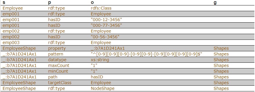
We load the two TriG files into our repository, and end up with the following triple set. Note that all the employee triples use the default graph and the SHACL-related triples use the graph <https://franz.com#Shapes> specified in the TriG file.

SHACL Triples

Now we use agtool shacl-validate to validate our data:

bin/agtool shacl-validate --data-graph default  --shapes-graph https://franz.com#Shapes shacl-repo-1  
Validation report:             Does not conform  
Created:                       2019-06-27T10:24:10  
Number of shapes graphs:       1  
Number of data graphs:         1  
Number of NodeShapes:          1  
Number of focus nodes checked: 3  
 
3 validation results:  
Result:  
 Focus node:           <https://franz.com#emp001>  
 Path:                 <https://franz.com#hasID>  
 Source Shape:         _:b7A1D241Ax1  
 Constraint Component: <http://www.w3.org/ns/shacl#MaxCountConstraintComponent>  
 Severity:             <http://www.w3.org/ns/shacl#Violation>  
 
Result:  
 Focus node:           <https://franz.com#emp002>  
 Path:                 <https://franz.com#hasID>  
 Value:                "00-56-3456"  
 Source Shape:         _:b7A1D241Ax1  
 Constraint Component: <http://www.w3.org/ns/shacl#PatternConstraintComponent>  
 Severity:             <http://www.w3.org/ns/shacl#Violation>  
 
Result:  
 Focus node:           <https://franz.com#emp003>  
 Path:                 <https://franz.com#hasID>  
 Source Shape:         _:b7A1D241Ax1  
 Constraint Component: <http://www.w3.org/ns/shacl#MinCountConstraintComponent>  
 Severity:             <http://www.w3.org/ns/shacl#Violation> 

The validation fails with the problems listed above. The Focus node is the subject of a triple that did not conform. Path is the predicate or a property path (predicates in this example). Value is the offending value. Source Shape is the shape that established the constraint (you must look at the shape triples to see exactly what Source Shape is requiring).

We revise our employee data with the following SPARQL expresssion, deleting one of the emp001 triples, deleting the emp002 triple and adding a new one with the correct format, and adding an emp003 triple.

prefix fr: <https://franz.com#>  
 
DELETE DATA {fr:emp002 fr:hasID "00-56-3456" } ;  
 
INSERT DATA {fr:emp002 fr:hasID "000-14-1772" } ;  
 
DELETE DATA {fr:emp001 fr:hasID "000-77-3456" } ;  
 
INSERT DATA {fr:emp003 fr:hasID "000-54-9662" } ; 

Now our employee triples are

SHACL Triples 2

We run the validation again and are told our data conforms:

% bin/agtool shacl-validate --data-graph default  --shapes-graph https://franz.com#Shapes shacl-repo-1  
Validation report:             Conforms  
Created:                       2019-06-27T10:32:19  
Number of shapes graphs:       1  
Number of data graphs:         1  
Number of NodeShapes:          1  
Number of focus nodes checked: 3 

When we refer to this example in the remainder of this document, it is to the un-updated (incorrect) triples.

SHACL API

The example above illustrates the SHACL steps:

  1. Have a data set with triples that should conform to a shape
  2. Have SHACL triples that express the desired shape
  3. Run SHACL validation to determine if the data conforms

Note that SHACL validation does not modify the data being validated. Once you have the conformance report, you must modify the data to fix the conformance problems and then rerun the validation test.

The main entry point to the API is agtool shacl-validate. It takes various options and has several output choices. Online help for agtool shacl-validate is displayed by running agtool shacl-validate --help.

In order to validate triples, the system must know:

  1. What tripes to examine
  2. What rules (SHACL triples) to use
  3. What to do with the results

Specifying what triples to examine

Two arguments to agtool shacl-validate specify the triples to evaluate: --data-graph and --focus-node. Each can be specified multiple times.

  • The --data-graph argument specifies the graph value for triples to be examined. Its value must be an IRI or default. Only triples in the specified graphs will be examined. default specifies the default graph. It is also the default value of the --data-graph argument. If no value is specified for --data-graph, only triples in the default graph will be examined. If a value for --data-graph is specified, triples in the default graph will only be examined if --data-graph default is also specified.
  • The --focus-node argument specifies IRIs which are subjects of triples. If this argument is specified, only triples with these subjects will be examined. To be examined, triples must also have graph values specified by --data-graph arguments. --focus-node does not have a default value. If unspecified, all triples in the specified data graphs will be examined. This argument can be specified multiple times.

The --data-graph argument was used in the simple example above. Here is how the --focus-node argument can be used to restrict validation to triples with subjects <https://franz.com#emp002>and <https://franz.com#emp003> and to ignore triples with subject <https://franz.com#emp001> (applying agtool shacl-validate to the orignal non-conformant data):

% bin/agtool shacl-validate --data-graph default  \  
  --shapes-graph https://franz.com#Shapes \  
  --focus-node https://franz.com#emp003 \  
  --focus-node https://franz.com#emp002 shacl-repo-1  
Validation report:             Does not conform  
Created:                       2019-06-27T11:37:49  
Number of shapes graphs:       1  
Number of data graphs:         1  
Number of NodeShapes:          1  
Number of focus nodes checked: 2  
 
2 validation results:  
Result:  
 Focus node:           <https://franz.com#emp003>  
 Path:                 <https://franz.com#hasID>  
 Source Shape:         _:b7A1D241Ax2  
 Constraint Component: <http://www.w3.org/ns/shacl#MinCountConstraintComponent>  
 Severity:             <http://www.w3.org/ns/shacl#Violation>  
 
Result:  
 Focus node:           <https://franz.com#emp002>  
 Path:                 <https://franz.com#hasID>  
 Value:                "00-56-3456"  
 Source Shape:         _:b7A1D241Ax2  
 Constraint Component: <http://www.w3.org/ns/shacl#PatternConstraintComponent>  
 Severity:             <http://www.w3.org/ns/shacl#Violation> 

Specifying What Shape Triples to Use

Two arguments to agtool shacl-validate, analogous to the two arguments for data described above, specify Shape triples to use. Further, following the SHACL spec, data triples with predicate <http://www.w3.org/ns/shacl#shapeGraph> also specify graphs containing Shape triples to be used.

The arguments to agtool shacl-validate are the following. Each may be specified multiple times.

  • The --shapes-graph argument specifies the graph value for shape triples to be used for SHACL validation. Its value must be an IRI or defaultdefault specifies the default graph. The --shapes-graph argument has no default value. If unspecified, graphs specified by data triples with the <http://www.w3.org/ns/shacl#shapeGraph> predicate will be used (they are used whether or not --shapes-graph has a value). If --shapes-graph has no value and there are no data triples with the <http://www.w3.org/ns/shacl#shapeGraph> predicate, the data graphs are used for shape graphs. (Shape triples have a known format and so can be identified among the data triples.)
  • The --shape argument specifies IRIs which are subjects of shape nodes. If this argument is specified, only shape triples with these subjects and subsiduary triples to these will be used for validation. To be included, the triples must also have graph values specified by the --shapes-graph arguments or specified by a data triple with the <http://www.w3.org/ns/shacl#shapeGraph> predicate. --shape does not have a default value. If unspecified, all shapes in the shapes graphs will be used.

Other APIs

There is a lisp API using the function validate-data-graph, defined next:

validate-data-graphdb  &key  data-graph-iri/s  shapes-graph-iri/s  shape/s  focus-node/s  verbose  conformance-only?

function

Perform SHACL validation and return a validation-report structure.

The validation uses data-graph-iri/s to construct the dataGraph. This can be a single IRI, a list of IRIs or NIL, in which case the default graph will be used. The shapesGraph can be specified using the shapes-graph-iri/s parameter which can also be a single IRI or a list of IRIs. If shape-graph-iri/s is not specified, the SHACL processor will first look to create the shapesGraph by finding triples with the predicate sh:shapeGraph in the dataGraph. If there are no such triples, then the shapesGraph will be assumed to be the same as the dataGraph.

Validation can be restricted to particular shapes and focus nodes using the shape/s and focus-node/s parameters. Each of these can be an IRI or list of IRIs.

If conformance-only? is true, then validation will stop as soon as any validation failures are detected.

You can use validation-report-conforms-p to see whether or not the dataGraph conforms to the shapesGraph (possibly restricted to just particular shape/s and focus-node/s).

The function validation-report-conforms-p returns t or nil as the validation struct returned by validate-data-graph does or does not conform.

validation-report-conforms-preport

function

Returns t or nil to indicate whether or not REPORT (a validation-report struct) indicates that validation conformed.

There is also a REST API. See HTTP reference.

Validation Output

The simple example above and the SHACL examples below show output from agtool validate-shacl. There are various output formats, specified by the --output option. Those examples use the plain format, which means printing results descriptively. Other choices include jsontrigtrixturtlenquadsrdf-n3rdf/xml, and ntriples. Here are the simple example (uncorrected) results using ntriples output:

% bin/agtool shacl-validate --output ntriples --data-graph default --shapes-graph https://franz.com#Shapes shacl-repo-1  
 
_:b271983AAx1 <http://www.w3.org/1999/02/22-rdf-syntax-ns#type> <http://www.w3.org/ns/shacl#ValidationReport> .  
_:b271983AAx1 <http://www.w3.org/ns/shacl#conforms> "false"^^<http://www.w3.org/2001/XMLSchema#boolean> .  
_:b271983AAx1 <http://purl.org/dc/terms/created> "2019-07-01T18:26:03"^^<http://www.w3.org/2001/XMLSchema#dateTime> .  
_:b271983AAx1 <http://www.w3.org/ns/shacl#result> _:b271983AAx2 .  
_:b271983AAx2 <http://www.w3.org/1999/02/22-rdf-syntax-ns#type> <http://www.w3.org/ns/shacl#ValidationResult> .  
_:b271983AAx2 <http://www.w3.org/ns/shacl#focusNode> <https://franz.com#emp001> .  
_:b271983AAx2 <http://www.w3.org/ns/shacl#resultPath> <https://franz.com#hasID> .  
_:b271983AAx2 <http://www.w3.org/ns/shacl#resultSeverity> <http://www.w3.org/ns/shacl#Violation> .  
_:b271983AAx2 <http://www.w3.org/ns/shacl#sourceConstraintComponent> <http://www.w3.org/ns/shacl#MaxCountConstraintComponent> .  
_:b271983AAx2 <http://www.w3.org/ns/shacl#sourceShape> _:b271983AAx3 .  
_:b271983AAx1 <http://www.w3.org/ns/shacl#result> _:b271983AAx4 .  
_:b271983AAx4 <http://www.w3.org/1999/02/22-rdf-syntax-ns#type> <http://www.w3.org/ns/shacl#ValidationResult> .  
_:b271983AAx4 <http://www.w3.org/ns/shacl#focusNode> <https://franz.com#emp002> .  
_:b271983AAx4 <http://www.w3.org/ns/shacl#resultPath> <https://franz.com#hasID> .  
_:b271983AAx4 <http://www.w3.org/ns/shacl#resultSeverity> <http://www.w3.org/ns/shacl#Violation> .  
_:b271983AAx4 <http://www.w3.org/ns/shacl#sourceConstraintComponent> <http://www.w3.org/ns/shacl#PatternConstraintComponent> .  
_:b271983AAx4 <http://www.w3.org/ns/shacl#sourceShape> _:b271983AAx3 .  
_:b271983AAx4 <http://www.w3.org/ns/shacl#value> "00-56-3456" .  
_:b271983AAx1 <http://www.w3.org/ns/shacl#result> _:b271983AAx5 .  
_:b271983AAx5 <http://www.w3.org/1999/02/22-rdf-syntax-ns#type> <http://www.w3.org/ns/shacl#ValidationResult> .  
_:b271983AAx5 <http://www.w3.org/ns/shacl#focusNode> <https://franz.com#emp003> .  
_:b271983AAx5 <http://www.w3.org/ns/shacl#resultPath> <https://franz.com#hasID> .  
_:b271983AAx5 <http://www.w3.org/ns/shacl#resultSeverity> <http://www.w3.org/ns/shacl#Violation> .  
_:b271983AAx5 <http://www.w3.org/ns/shacl#sourceConstraintComponent> <http://www.w3.org/ns/shacl#MinCountConstraintComponent> .  
_:b271983AAx5 <http://www.w3.org/ns/shacl#sourceShape> _:b271983AAx3 . 

You can have the triples added to the repository by specifying the --add-to-repo option true.

In the plain output information is provided about how many data graphs are examined, how many shape graphs were specified and node shapes are found, and how many focus nodes are checked. If zero focus nodes are checked, that is likely not what you want and something has gone wrong. Here we mis-spell the name of the shape graph (https://franz.com#shapes instead of https://franz.com#Shapes) and get 0 focus nodes checked:

% bin/agtool shacl-validate --data-graph default --shapes-graph https://franz.com#shapes shacl-repo-1  
Validation report:             Conforms  
Created:                       2019-06-28T10:34:22  
Number of shapes graphs:       1  
Number of data graphs:         1  
Number of NodeShapes:          0  
Number of focus nodes checked: 0  

SPARQL integration

There are two sets of magic properties defined: one checks for basic conformance and the other produces validation reports as triples:

  • ?valid franz:shaclConforms ( ?dataGraph [ ?shapesGraph ] )
  • ?valid franz:shaclFocusNodeConforms1 ( ?dataGraph ?nodeOrNodeCollection )
  • ?valid franz:shaclFocusNodeConforms2 ( ?dataGraph ?shapesGraph ?nodeOrNodeCollection )
  • ?valid franz:shaclShapeConforms1 ( ?dataGraph ?shapeOrShapeCollection [ ?nodeOrNodeCollection ] )
  • ?valid franz:shaclShapeConforms2 ( ?dataGraph ?shapesGraph ?shapeOrShapeCollection [ ?nodeOrNodeCollection ] )
  • (?s ?p ?o) franz:shaclValidationReport ( ?dataGraph [ ?shapesGraph ] )
  • (?s ?p ?o) franz:shaclFocusNodeValidationReport1 ( ?dataGraph ?nodeOrNodeCollection ) .
  • (?s ?p ?o) franz:shaclFocusNodeValidationReport2 ( ?dataGraph ?shapesGraph ?nodeOrNodeCollection ) .
  • (?s ?p ?o) franz:shaclShapeValidationReport1 ( ?dataGraph ?shapeOrShapeCollection [ ?nodeOrNodeCollection ] ) .
  • (?s ?p ?o) franz:shaclShapeValidationReport2 ( ?dataGraph ?shapesGraph ?shapeOrShapeCollection [ ?nodeOrNodeCollection ] ) .

In all of the above ?dataGraph and ?shapesGraph can be IRIs, the literal ‘default’, or a variable that is bound to a SPARQL collection (list or set) that was previously created with a function like https://franz.com/ns/allegrograph/6.5.0/fn#makeSPARQLList or https://franz.com/ns/allegrograph/6.5.0/fn#lookupRdfList. If a collection is used, then the SHACL processor will create a temporary RDF merge of all of the graphs in it to produce the data graph or the shapes graph.

Similarly, ?shapeOrShapeCollection and ?nodeOrNodeCollection can be bound to an IRI or a SPARQL collection. If a collection is used, then it must be bound to a list of IRIs. The SHACL processor will restrict validation to the shape(s) and focus node(s) (i.e. nodes that should be validated) specified.

The shapesGraph argument is optional in both of the shaclConforms and shaclValidationReport magic properties. If the shapesGraph is not specified, then the shapesGraph will be created by following triples in the dataGraph that use the sh:shapesGraph predicate. If there are no such triples, then the shapesGraph will be the same as the dataGraph.

For example, the following SPARQL expression

construct { ?s ?p ?o } where {  
  # form a collection of focusNodes  
  bind(<https://franz.com/ns/allegrograph/6.6.0/fn#makeSPARQLList>(  
    <http://Journal1/1942/Article25>,  
    <http://Journal1/1943>) as ?nodes)  
  (?s ?p ?o) <https://franz.com/ns/allegrograph/6.6.0/shaclShapeValidationReport1>  
    ('default' <ex://franz.com/documentShape1> ?nodes) .  
} 

would use the default graph as the Data Graph and the Shapes Graph and then validate two focus nodes against the shape <ex://franz.com/documentShape1>.

SHACL Example

We build on our simple example above. Start with a fresh repository so triples from the simple example do not interfere with this example.

We start with a TriG file with various shapes defined on some classes.

@prefix sh: <http://www.w3.org/ns/shacl#> .  
@prefix xsd: <http://www.w3.org/2001/XMLSchema#> .  
@prefix fr: <https://franz.com#> .  
@prefix rdf: <http://www.w3.org/1999/02/22-rdf-syntax-ns#> .  
@prefix rdfs: <http://www.w3.org/2000/01/rdf-schema#> .  
 
<https://franz.com#ShapesGraph> {  
fr:EmployeeShape  
   a sh:NodeShape ;  
   sh:targetClass fr:Employee ;  
   sh:property [  
     ## Every employee must have exactly one ID  
     sh:path fr:hasID ;  
     sh:minCount 1 ;  
     sh:maxCount 1 ;  
     sh:datatype xsd:string ;  
     sh:pattern "^[0-9][0-9][0-9]-[0-9][0-9]-[0-9][0-9][0-9][0-9]$" ;  
    ] ;  
   sh:property [  
     ## Every employee is a manager or a worker  
     sh:path fr:employeeType ;  
     sh:minCount 1 ;  
     sh:maxCount 1 ;  
     sh:datatype xsd:string ;  
     sh:in ("Manager" "Worker") ;  
    ] ;  
    sh:property [  
      ## If birthyear supplied, must be 2001 or before  
      sh:path fr:birthYear ;  
      sh:maxInclusive 2001 ;  
      sh:datatype xsd:integer ;  
    ] ;  
    sh:property [  
      ## Must have a title, may have more than one  
      sh:path fr:hasTitle ;  
      sh:datatype xsd:string ;  
      sh:minCount 1 ;  
    ] ;  
 
    sh:or (  
      ## The President does not have a supervisor  
      [  
        sh:path fr:hasTitle ;  
        sh:hasValue "President" ;  
      ]  
      [  
       ## Must have a supervisor  
         sh:path fr:hasSupervisor ;  
         sh:minCount 1 ;  
         sh:maxCount 1 ;  
         sh:class fr:Employee ;  
      ]  
      ) ;  
 
    sh:or (  
      # Every employee must either have a wage or a salary  
      [  
       sh:path fr:hasSalary ;  
       sh:datatype xsd:integer ;  
       sh:minInclusive 3000 ;  
       sh:minCount 1 ;  
       sh:maxCount 1 ;  
      ]  
      [  
       sh:path fr:hasWage ;  
       sh:datatype xsd:decimal ;  
       sh:minExclusive 15.00 ;  
       sh:minCount 1 ;  
       sh:maxCount 1 ;  
      ]  
    )  
    .  
   } 

This file says the following about instances of the class fr:Employee:

  1. Every employee must have exactly one ID (object of fr:hasID), a string of the form NNN-NN-NNNN where the Ns are digits (this is the simple example requirement).
  2. Every employee must have exactly one fr:employeeType triple with value either “Manager” or “Worker”.
  3. Employees may have a fr:birthYear triple, and if so, the value must be 2001 or earlier.
  4. Employees must have a fr:hasTitle and may have more than one.
  5. All employees except the one with title “President” must have a supervisor (specified with fr:hasSupervisor).
  6. Every employee must either have a wage (a decimal specifying hourly pay, greater than 15.00) or a salary (an integer specifying monthly pay, greater than or equal to 3000).

Here is some employee data:

@prefix fr: <https://franz.com#> .  
@prefix rdf: <http://www.w3.org/1999/02/22-rdf-syntax-ns#> .  
@prefix rdfs: <http://www.w3.org/2000/01/rdf-schema#> .  
@prefix xsd: <http://www.w3.org/2001/XMLSchema#> .  
 
{  
 fr:Employee  
  a rdfs:Class .  
 
 fr:emp001  
  a fr:Employee ;  
  fr:hasID "000-12-3456" ;  
  fr:hasTitle "President" ;  
  fr:employeeType "Manager" ;  
  fr:birthYear "1953"^^xsd:integer ;  
  fr:hasSalary "10000"^^xsd:integer .  
 
 fr:emp002  
  a fr:Employee ;  
  fr:hasID "000-56-3456" ;  
  fr:hasTitle "Foreman" ;  
  fr:employeeType "Worker" ;  
  fr:birthYear "1966"^^xsd:integer ;  
  fr:hasSupervisor fr:emp003 ;  
  fr:hasWage "20.20"^^xsd:decimal .  
 
 fr:emp003  
  a fr:Employee ;  
  fr:hasID "000-77-3232" ;  
  fr:hasTitle "Production Manager" ;  
  fr:employeeType "Manager" ;  
  fr:birthYear "1968"^^xsd:integer ;  
  fr:hasSupervisor fr:emp001 ;  
  fr:hasSalary "4000"^^xsd:integer .  
 
 fr:emp004  
  a fr:Employee ;  
  fr:hasID "000-88-3456" ;  
  fr:hasTitle "Fitter" ;  
  fr:employeeType "Worker" ;  
  fr:birthYear "1979"^^xsd:integer ;  
  fr:hasSupervisor fr:emp002 ;  
  fr:hasWage "17.20"^^xsd:decimal .  
 
 fr:emp005  
  a fr:Employee ;  
  fr:hasID "000-99-3492" ;  
  fr:hasTitle "Fitter" ;  
  fr:employeeType "Worker" ;  
  fr:birthYear "2000"^^xsd:integer ;  
  fr:hasWage "17.20"^^xsd:decimal .  
 
 fr:emp006  
  a fr:Employee ;  
  fr:hasID "000-78-5592" ;  
  fr:hasTitle "Filer" ;  
  fr:employeeType "Intern" ;  
  fr:birthYear "2003"^^xsd:integer ;  
  fr:hasSupervisor fr:emp002 ;  
  fr:hasWage "14.20"^^xsd:decimal .  
 
 fr:emp007  
  a fr:Employee ;  
  fr:hasID "000-77-3232" ;  
  fr:hasTitle "Sales Manager" ;  
  fr:hasTitle "Vice President" ;  
  fr:employeeType "Manager" ;  
  fr:birthYear "1962"^^xsd:integer ;  
  fr:hasSupervisor fr:emp001 ;  
  fr:hasSalary "7000"^^xsd:integer .  
 } 

Comparing these data with the requirements, we see these problems:

  1. emp005 does not have a supervisor.
  2. emp006 is pretty messed up, with (1) employeeType “Intern”, not an allowed value, (2) a birthYear (2003) later than the required maximum of 2001, and (3) a wage (14.40) less than the minimum (15.00).

Otherwise the data seems OK.

We load these two TriG files into an emply repository (which we have named shacl-repo-2). We specify the default graph for the data and the https://franz.com#ShapesGraph for the shapes. (Though not required, it is a good idea to specify a graph for shape data as it makes it easy to delete and reload shapes while developing.) We have 101 triples, 49 data and 52 shape. Then we run agtool shacl-validate:

% bin/agtool shacl-validate --shapes-graph https://franz.com#ShapesGraph --data-graph default shacl-repo-2 

There are four violations, as expected, one for emp005 and three for emp006.

Validation report:             Does not conform  
Created:                       2019-07-03T11:35:27  
Number of shapes graphs:       1  
Number of data graphs:         1  
Number of NodeShapes:          1  
Number of focus nodes checked: 7  
 
4 validation results:  
Result:  
 Focus node:           <https://franz.com#emp005>  
 Value:                <https://franz.com#emp005>  
 Source Shape:         <https://franz.com#EmployeeShape>  
 Constraint Component: <https://www.w3.org/ns/shacl#OrConstraintComponent>  
 Severity:             <https://www.w3.org/ns/shacl#Violation>  
 
Result:  
 Focus node:           <https://franz.com#emp006>  
 Path:                 <https://franz.com#employeeType>  
 Value:                "Intern"  
 Source Shape:         _:b19D062B9x221  
 Constraint Component: <http://www.w3.org/ns/shacl#InConstraintComponent>  
 Severity:             <http://www.w3.org/ns/shacl#Violation>  
 
Result:  
 Focus node:           <https://franz.com#emp006>  
 Path:                 <https://franz.com#birthYear>  
 Value:                "2003"^^<http://www.w3.org/2001/XMLSchema#integer>  
 Source Shape:         _:b19D062B9x225  
 Constraint Component: <http://www.w3.org/ns/shacl#MaxInclusiveConstraintComponent>  
 Severity:             <http://www.w3.org/ns/shacl#Violation>  
 
Result:  
 Focus node:           <https://franz.com#emp006>  
 Value:                <https://franz.com#emp006>  
 Source Shape:         <https://franz.com#EmployeeShape>  
 Constraint Component: <http://www.w3.org/ns/shacl#OrConstraintComponent>  
 Severity:             <http://www.w3.org/ns/shacl#Violation>  

Fixing the data is left as an exercise for the reader.


AllegroGraph Named to DBTA Top 100 That Matter Most in Data

Franz Inc., an early innovator in Artificial Intelligence (AI) and leading supplier of Graph and Document Database technology for Knowledge Graphs, today announced that it has been named to Database Trends and Applications (DBTA) – 2019 Top 100 That Matter Most in Data.

“We’re excited to announce our seventh annual list, as the industry continues to grow and evolve,” remarked Thomas Hogan, Group Publisher at Database Trends and Applications. “Today, more than ever, businesses are looking to increase their efficiency, agility and ability to innovate by managing and leveraging data in new and novel ways. This list seeks to highlight those companies that have been successful in establishing themselves as unique resources for data professionals and stakeholders.”

“We are honored to receive this acknowledgement for our efforts in delivering Enterprise Knowledge Graph Solutions,” said Dr. Jans Aasman, CEO, Franz Inc. “In the past year, we have seen demand for Enterprise Knowledge Graphs take off across industries along with recognition from top technology analyst firms that Knowledge Graphs provide the critical foundation for artificial intelligence applications and predictive analytics. Our AllegroGraph Knowledge Graph Platform Solution offers a unique comprehensive approach for helping companies accelerate the creation of Enterprise Knowledge Graphs that deliver new value to their organization.”

Franz’s Knowledge Graph Platform Solution includes both technology and services for building industrial strength Knowledge Graphs based on best-of-class tools, products, knowledge, skills and experience. At the core of the solution is Franz’s graph database technology, AllegroGraph, which is utilized by dozens of the top F500 companies worldwide and enables businesses to extract sophisticated decision insights and predictive analytics from highly complex, distributed data that cannot be uncovered with conventional databases.

Franz delivers the expertise for designing ontology and taxonomy-based solutions by utilizing standards-based development processes and tools. Franz also offers data integration services from siloed data using W3C industry standard semantics, which can then be continually integrated with information that comes from other data sources. In addition, the Franz data science team provides expertise in custom algorithms to maximize data analytics and uncover hidden knowledge.

Companies Across the Globe Use Franz Knowledge Graph Solutions

Organizations in customer service, healthcare, life science, publishing and technology have relied on Franz to help develop their knowledge graph solutions.

Global B2B technology firm N3 Results has utilized Franz’s Knowledge Graph Solution to build an ‘Intelligent Sales Organization,’ which uses graph based technology for taxonomy driven entity extraction, speech recognition, machine learning and predictive analytics to improve quality of conversations, increase sales and improve business visibility.

“In a typical sales organization, the valuable content within the online chat or voice conversation between the agent and customer goes into a black hole,” said Shannon Copeland, COO of N3. “Franz helped us build a modern Intelligent Sales Organization (ISO) by creating a real-time Knowledge Graph that knows everything about customers and agents and provides the raw data for machine learning to improve doing the business of ISO. Now we use the rich information between agents and customers to improve the quality of the interaction in real time, which ultimately creates more sales and provides far better analytics for management.”

In 2015, Dr. Parsa Mirhaji, his colleagues and industry partners, including Franz Inc. embarked on a project to bring Knowledge Graph technology to Montefiore, a Bronx-based medical center. “Our strategy at Montefiore is to build a data-driven and evidence-based health system – essentially a learning healthcare system – that can understand its own population thoroughly, understand and improve its practices, and develop the highest quality of services for the people it serves,” said Parsa Mirhaji, MD, PhD, Director of the Center for Health Data Innovations at Montefiore and the Albert Einstein College of Medicine. “In order to accomplish that goal, we have created a system that harvests every piece of data that we can possibly find, from our own EMRs and devices to patient-generated data to socioeconomic data from the community. It’s extremely important to use anything we can find that can help us categorize our patients more accurately.” (Health IT Analytics, At Montefiore, Artificial Intelligence Becomes Key to Patient Care, September 10, 2018)

Wolters Kluwer is using graph analytic techniques to accelerate the knowledge discovery process for its clients. “What we’re really interested in is achieving insights that today take a person to analyze and that are prohibitive computationally,” said Greg Tatham, Wolters Kluwer CTO of Global Platforms. “We’re providing this live feedback. As you’re typing, we’re providing question and suggestions for you live. AllegroGraph gives us a performant way to be able to just work our way through the whole knowledge model and come up with suggestions to the user in real time.” (Datanami, How AI Boosts Human Expertise at Wolters Kluwer, June 6, 2018)

Gartner Identifies Knowledge Graphs and Semantics as Key Technologies for AI
Gartner recently recognized knowledge graphs as a key new technology in both their Hype Cycle for Artificial Intelligence and Hype Cycle for Emerging Technologies. Gartner’s Hype Cycle for Artificial Intelligence 2018 states, “The rising role of content and context for delivering insights with AI technologies, as well as recent knowledge graph offerings for AI applications have pulled knowledge graphs to the surface.”

Semantics has also been identified by Gartner as critical for effectively utilizing enterprise data assets. “Unprecedented levels of data scale and distribution are making it almost impossible for organizations to effectively exploit their data assets. Data and analytics leaders must adopt a semantic approach to their enterprise data assets or face losing the battle for competitive advantage.” (Gartner, How to Use Semantics to Drive the Business Value of Your Data, Guido De Simoni, November 27, 2018) For more information about the Gartner report, visit the Gartner Report Order Page.

About Franz Inc.
Franz Inc. is an early innovator in Artificial Intelligence (AI) and leading supplier of Semantic Graph Database technology with expert knowledge in developing and deploying Knowledge Graph solutions. The foundation for Knowledge Graphs and AI lies in the facets of semantic technology provided by AllegroGraph and Allegro CL. The ability to rapidly integrate new knowledge is the crux of the Knowledge Graph and Franz Inc. provides the key technologies and services to address your complex challenges. Franz Inc. is your Knowledge Graph technology partner.

About Database Trends and Applications
Database Trends and Applications (DBTA), published by Information Today, Inc., is a bimonthly magazine that delivers advanced trends analysis and case studies in data management and analysis developed by a team with more than 25 years of industry experience. Visit www.dbta.com for subscription information. DBTA also delivers groundbreaking market research exclusively through its Unisphere Research group.


Creating Explainable AI With Rules

Franz’s CEO, Jans Aasman’s recent Forbes article:

There’s a fascinating dichotomy in artificial intelligence between statistics and rules, machine learning and expert systems. Newcomers to artificial intelligence (AI) regard machine learning as innately superior to brittle rules-based systems, while  the history of this field reveals both rules and probabilistic learning are integral components of AI.

This fact is perhaps nowhere truer than in establishing explainable AI, which is central to the long-term business value of AI front-office use cases.

Granted, simple machine learning can automate backend processes. However, the full extent of deep learning or complex neural networks — which are much more accurate than basic machine learning — for mission-critical decision-making and action requires explainability.

Using rules (and rules-based systems) to explicate machine learning results creates explainable AI. Many of the far-reaching applications of AI at the enterprise level — deploying it to combat financial crimes, to predict an individual’s immediate and long-term future in health care, for example — require explainable AI that’s fair, transparent and regulatory compliant.

Rules can explain machine learning results for these purposes and others.

Read the full article at Forbes


Adding Properties to Triples in AllegroGraph

AllegroGraph provides two ways to add metadata to triples. The first one is very similar to what typical property graph databases provide: we use the named graph of triples to store meta data about that triple. The second approach is what we have termed triple attributes. An attribute is a key/value pair associated with an individual triple. Each triple can have any number of attributes. This approach, which is built into AllegroGraph’s storage layer, is especially handy for security and bookkeeping purposes. Most of this article will discuss triple attributes but first we quickly discuss the named graph (i.e. fourth element or quad) approach.

1.0 The Named Graph for Properties

Semantic Graph Databases are actually defined by the W3C standard to store RDF as ‘Quads’ (Named Graph, Subject, Predicate, and Object).  The ‘Triple Store’ terminology has stuck even though the industry has moved on to storing quads.   We believe using the named graph approach to store metadata about triples is richer model that the property graph database method.

The best way to understand this is to give an example. Below we see two statements about Bruce weighing 105 kilos. The triple portions (subject, predicate, object) are identical but the named graphs (fourth elements) differ. They are used to provide additional information about the triples. The graph values are S1 and S2. By looking at these graphs we see that

  • The author of the first triple (with graph S1) is Sophia and the author of the second (with graph S2) is Bruce (who is also the subject of the two triples).
  • Sophia is 100% certain about her statement while Bruce is only 10% certain about his.

Using the named graph we can do even more than a property graph database, as the value of a graph can itself be a node, and is the subject of various triples which specify the original triple’s author, date, and certainty. Additional triples tell us the ages of the authors and the fact that the authors are married.

Here is the data displayed in Gruff, AllegroGraph’s associated triple store browser:

Using named graphs for a  triple’s metadata is a powerful tool but it does have limitations: (1) only one graph value can be associated with a triple, (2) it can be important that metadata is stored directly and physically with the triple (with named graphs, the actual metadata is usually stored in additional triples with the graph as the subject, as in the example above), and (3) named graphs have competing uses and may not be available for metadata.

2.0 The Triple Attributes approach

AllegroGraph uniquely offers a mechanism called triple attributes where a collection of user defined key/value pairs can be stored with each individual triple. The advantage of this approach is manyfold, but the original use case was designed for triple level security for an Intelligence agency.

By having triple attributes physically connected to the triples in the storage layer we can provide a very powerful and flexible mechanism to protect triples at the lowest possible level in AllegroGraph’s architecture. Our first example below shows this use case in great detail. Other use cases are for example to add weights or costs to triples, to be used in graph algorithms. Or we can add a recorded time or expiration times to a triple and use that to provide a time machine in AllegroGraph or do automatic clean-up of old data.

Example with Attributes:

      Subject – <http://dbpedia.org/resource/Arif_Babayev>
      Predicate – <http://dbpedia.org/property/placeOfDeath>
      Object – <http://dbpedia.org/resource/Baku>
      Named Graph – <http://ex#trans@@1142684573200001>
      Triple Attributes – {“securityLevel”: “high”, “department”: “hr”, “accessToken”: [“E”, “D”]}

This article provides an initial introduction to attributes and the associated concept of static filters, showing how they are set up and used. We start with a security example which also describes the basics of adding attributes to triples and filtering query results based on attribute values. Then we discuss other potential uses of attributes.

2.1 Triple Attribute Basics: a Security Example

One important purpose of attributes, when they were added as a feature, was to allow for very fine triple-level security, so that triples would be visible or invisible to users according to the attributes of the triples and the permissions associated with the query being posed by the user.

Note that users as such do not have attributes. Instead, attribute values are assigned when a query is posed. This is an important point: it is natural to think that there can be an attribute SECURITY-LEVEL, and a triple can have attribute SECURITY-LEVEL=3, and USER1 can have an attribute SECURITY-LEVEL=2 and USER2 can have an attribute SECURITY-LEVEL=4, and the system can require that the user SECURITY-LEVEL attribute must be greater than the triple SECURITY-LEVEL for the triple to be visible to the user. But that is not how attributes work. The triples can have the attribute SECURITY-LEVEL=2 but users do not have attributes. Instead, the filter is made part of the query.

Here is a simple example. We define attributes and static attribute filters using AGWebView. We have a repository named repo. Here is a portion of its AGWebView page:

The red arrow points to the commands of interest: Manage attribute definitions and Set static attribute filter. We click on Set static attribute filter to define an attribute. We have filled in the attribute information (name security-level, minimum and maximum number allowed per triple, allowed values, and whether order or not (yes in our case):

We click Save and the attribute is defined:

Then we define a filter (on the Set static attribute filter page):

We defined the filter (attribute-set> user.security-level triple.security-level) and clicked Save (the definition appears in both the Edit and the Current fields). The filter says that the “user” security level must be greater than the triple security level. We put “user” in quotes because the user security level is specified as part of the query, and has no direct connection to any specific user.

Here are some triples in a nqx file fr.nqx. The first triple has no attributes and the other three each has a security-level attribute value.

     <http://www.franz.com#emp0> <http://www.franz.com#position> “intern” .

     <http://www.franz.com#emp1> <http://www.franz.com#position> “worker” {“security-level”: “2”} .

     <http://www.franz.com#emp2> <http://www.franz.com#position> “manager” {“security-level”: “3”} .

     <http://www.franz.com#emp3> <http://www.franz.com#position> “boss” {“security-level”: “4”} .

We load this file into a repository which has the security-level attribute defined as above and the static filter mentioned above also defined. (Triples with attributes can also be entered directly when using AGWebView with the Import RDF from a text area input command).

Once the triples are loaded, we click View triples in AGWebView and we see no triples:

This result is often surprising to users just beginning to work with attributes and filters, who may expect the first triple, abbreviated to [emp0 position intern], to be visible, but the system is doing what it is supposed to do. It will only show triples where the security-level of the user posing the query is greater than the security level of the triple. The user has no security level and so the comparison fails, even with triples that have no security-level attribute value. We will describe below how to ensure you can see triples with no attributes.

So we need to specify an attribute value to the user posing the query. (As said above, users do not themselves have attribute values. But the attribute value of a user posing a query can be specified as part of the query.) “User” attributes are specified with a prefix like the following:

     prefix franzOption_userAttributes: <franz:%7B%22security-level%22%3A%223%22%7D>

so the query should be

     prefix franzOption_userAttributes: <franz:%7B%22security-level%22%3A%223%22%7D>

     select ?s ?p ?o { ?s ?p ?o . }

We will show the results below, but first what are all the % signs and numbers doing there? Why isn’t the prefix just prefix franzOption_userAttributes: <franz:{“security-level”:”3″}>? The issue is that {“security-level”:”3″} won’t read correctly. It must be URL encoded. We do this by going to https://www.urlencoder.org/ (there are other websites that do this as well) and put {“security-level”:”3″} in the first box, click Encode and get %7B%22security-level%22%3A%223%22%7D.  We then paste that into the query, as shown above.

When we try that query in AGWebView, we get one result:

If we encode {“security-level”:”5″} to get the query

prefix franzOption_userAttributes: <franz:%7B%22security-level%22%3A%225%22%7D>
select ?s ?p ?o { ?s ?p ?o . }

we get three results:

     emp3    position                “boss”
     emp2    position                “manager”
     emp1    position                “worker”

since now the “user” security-level is greater than that of any triples with a security-level attribute. But what about the triple with subject emp0, the triple with no attributes? It does not pass the filter which required that the user attribute be greater than the triple attribute. Since the triple has no attribute value so the comparison failed.

Let us redefine the filter to:

(or (attribute-set> user.security-level triple.security-level)
    (empty triple.security-level))

Now a triple will pass the filter if either (1) the “user” security-level is greater than the triple security-level or (2) the triple does not have a security-level attribute. Now the query from above where the user has attribute security-level:”5” will show all the triples with security-level less than 5 and with no attributes at all. That happens to be all four triples so far defined:

The triple

     emp0    position                “intern”

will now appears as a result in any query where it satisfies the SPARQL select regardless of the security-level of the “user”.

It would be a useful feature that we could associate attributes with actual users. However, this is not as simple as it sounds. Attributes are features of repositories. If I have a REPO1 repository, it can have a bunch of defined attributes and filters but my REPO2 may know nothing about them and its triples may not have any attributes at all, and no attributes are defined, and (as a result) no filters. But users are not repository-linked objects. While a repository can be made read-only or unreadable for a user, users do not have finer repository features. So an interface for providing users with attributes, since it would only make sense on a per-repository basis, requires a complicated interface. That is not yet implemented (though we are considering how it can be done).

Instead, users can have specific prefixes associated with them and that prefix and be included in any query made by the user.

But if all it takes to specify “user” attributes is to put the right line at the top of your SPARQL query, that does not seem to provide much security. There is a feature for users “Allow user attributes via SPARQL PREFIX franzOption_userAttributes” which can restrict a user’s ability to specify “user” attributes in a query, but that is a rather blunt instrument. Instead, the model is that most users (outside of trusted administrators) are not actually allowed to pose SPARQL queries directly. Instead, there is an intermediary program which takes the query a user requests and, having determined the status of the user and what attribute values should be given to the user, modifies the query with the appropriate franzOption_userAttributes prefixes and then sends the query on to the server, following which it captures the results and sends them back to the requesting user. That intermediate program will store the prefix suitable for a user and thus associate “user” attributes with specific users.

2.2 Using attributes as additional data

Although triple security is one powerful use of attributes, security is far from the only use. Just as the named graph can serve as additional data, so can attributes. SPARQL queries can use attribute values just as static filters can filter out triples before displaying them. Let us take a simple example: the attribute timeAdded. Every triple we add will have a timeAdded attribute value which will be a string whose contents are a datetime value, such as “2017-09-11T:15:52”. We define the attribute:

Now let us define some triples:

     <http://www.franz.com#emp0> <http://www.franz.com#callRank> “2” {“timeAdded”: “2019-01-12T10:12:45” } .
     <http://www.franz.com#emp0> <http://www.franz.com#callRank> “1” {“timeAdded”: “2019-01-14T14:16:12” } .
     <http://www.franz.com#emp0> <http://www.franz.com#callRank> “3” {“timeAdded”: “2019-01-11T11:15:52” } .
     <http://www.franz.com#emp1> <http://www.franz.com#callRank> “5” {“timeAdded”: “2019-01-13T11:03:22” } .
     <http://www.franz.com#emp0> <http://www.franz.com#callRank> “2” {“timeAdded”: “2019-01-13T09:03:22” } .


We have a call center with employees making calls. Each call has a ranking from 1 to 5, with 1 the lowest and 5 the highest. We have data on five calls, four from emp0 and one from emp1. Each triples has a timeAdded attribute with a string containing a dateTime value. We load these into a empty repository named at-test where the timeAdded attribute is defined as above:


SPARQL queries can use the attribute magic properties (see https://franz.com/agraph/support/documentation/current/triple-attributes.html#Querying-Attributes-using-SPARQL). We use the attributesNameValue magic property to see the subject, object, and attribute value:

     select ?s ?o ?value { 
       (?ta ?value) <http://franz.com/ns/allegrograph/6.2.0/attributesNameValue>    (?s ?p ?o) . 
     }

But we are really interested just in emp0 and we would like to see the results ordered by time, that is by the attribute value, so we restrict the query to emp0 as the subject and order the results:

     select ?o ?value { 
       (?ta ?value) <http://franz.com/ns/allegrograph/6.2.0/attributesNameValue>    (<http://www.franz.com#emp0> ?p ?o) . 
     }  order by ?value

There are the results for emp0, who is clearly having difficulties because the call rankings have been steadily falling over time.

Another example using timeAdded is employee salary data. In the Human Resources data, the salary of an employee is stored:

      emp0 hasSalary 50000

Now emp0 gets a raise to 55000. So we delete the triple above and add the triple

      emp0 hasSalary 55000

But that is not satisfactory because we have lost the salary history. If the boss asks “How much was emp0 paid initially?” we cannot answer. There are various solutions. We could define a salary change object, with predicates effectiveDate, previousSalary, newSalary, and so on:

     salaryChange017 forEmployee emp0
     salaryChange017 effectiveDate “2019-01-12T10:12:45”
     salaryChange017 oldSalary “50000”
     salaryChange017 newSalary “55000”

     emp0 hasSalaryChange salaryChange017

and that would work fine, but perhaps it is more setup and effort than is needed. Suppose we just have hasSalary triples each with a timeAdded attribute. Then the current salary is the latest one and the history is the ordered list. Here that idea is worked out:

<http://www.franz.com#emp0> <http://www.franz.com#hasSalary> “50000”^^<http://www.w3.org/2001/XMLSchema#integer> {“timeAdded”: “2017-01-12T10:12:45” } .
<http://www.franz.com#emp0> <http://www.franz.com#hasSalary> “55000”^^<http://www.w3.org/2001/XMLSchema#integer> {“timeAdded”: “2019-03-17T12:00:00” } .

What is the current salary? A simple SPARQL query tells us:

      select ?o ?value { 
       (?ta ?value) <http://franz.com/ns/allegrograph/6.2.0/attributesNameValue>  
                       (<http://www.franz.com#emp0> <http://www.franz.com#hasSalary> ?o) . 
        }  order by desc(?value) limit 1


The salary history is provided by the same query without the LIMIT:

     select ?o ?value { 
       (?ta ?value) <http://franz.com/ns/allegrograph/6.2.0/attributesNameValue>   
                      (<http://www.franz.com#emp0> <http://www.franz.com#hasSalary> ?o) . 
        }  order by desc(?value)


This method of storing salary data may not easily support more complex questions which might be easily answered if we went the salaryChange object route mentioned above but if you are not looking to ask those questions, you should not do the extra work (and the risk of data errors) required.

You could use the graph of each triple for the timeAdded. All the examples above would work with minor tweaks. But there are many uses for the named graph of a triple. Attributes are available and using them for one purpose does not restrict their use for other purposes.


Using JSON-LD in AllegroGraph – Python Example

The following is example #19 from our AllegroGraph Python Tutorial.
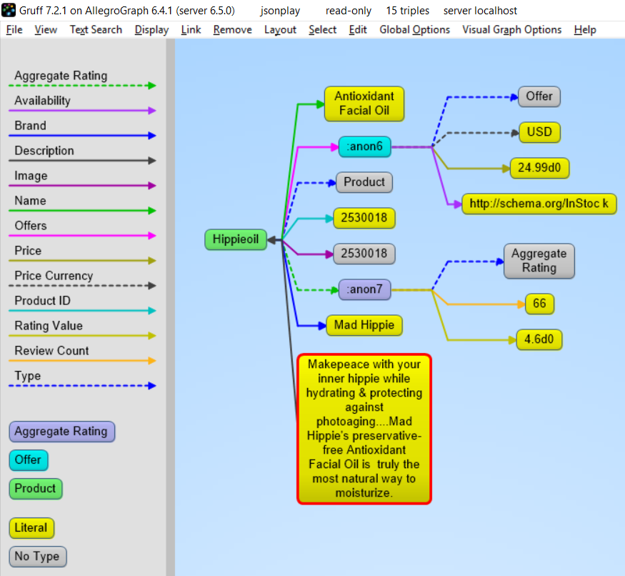
JSON-LD is described pretty well at https://json-ld.org/ and the specification can be found at https://json-ld.org/latest/json-ld/ .

The website https://json-ld.org/playground/ is also useful.

There are many reasons for working with JSON-LD. The major search engines such as Google require ecommerce companies to mark up their websites with a systematic description of their products and more and more companies use it as an easy serialization format to share data.

The benefit for your organization is that you can now combine your documents with graphs, graph search and graph algorithms. Normally when you store documents in a document store you set up your documents in such a way that it is optimized for direct retrieval queries. Doing complex joins for multiple types of documents or even doing a shortest path through a mass of object (types) is however very complicated. Storing JSON-LD objects in AllegroGraph gives you all the benefits of a document store and you can semantically link objects together, do complex joins and even graph search.

A second benefit is that, as an application developer, you do not have to learn the entire semantic technology stack, especially the part where developers have to create individual triples or edges. You can work with the JSON data serialization format that application developers usually prefer.

In the following you will first learn about JSON-LD as a syntax for semantic graphs. After that we will talk more about using JSON-LD with AllegroGraph as a document-graph-store.

Setup

You can use Python 2.6+ or Python 3.3+. There are small setup differences which are noted. You do need agraph-python-101.0.1 or later.

Mimicking instructions in the Installation document, you should set up the virtualenv environment.

  1. Create an environment named jsonld:
python3 -m venv jsonld

or

python2  -m virtualenv jsonld

  1. Activate it:

Using the Bash shell:

source jsonld/bin/activate

Using the C shell:

source jsonld/bin/activate.csh
  1. Install agraph-python:
pip install agraph-python

And start python:

python
[various startup and copyright messages]
>>>

We assume you have an AllegroGraph 6.5.0 server running. We call ag_connect. Modify the hostportuser, and password in your call to their correct values:

from franz.openrdf.connect import ag_connect
with ag_connect('repo', host='localhost', port='10035',
                user='test', password='xyzzy') as conn:
    print (conn.size())

If the script runs successfully a new repository named repo will be created.

JSON-LD setup

We next define some utility functions which are somewhat different from what we have used before in order to work better with JSON-LD. createdb() creates and opens a new repository and opendb() opens an existing repo (modify the values of hostportuser, and password arguments in the definitions if necessary). Both return repository connections which can be used to perform repository operations. showtriples() displays triples in a repository.

import os
import json, requests, copy

from franz.openrdf.sail.allegrographserver import AllegroGraphServer
from franz.openrdf.connect import ag_connect
from franz.openrdf.vocabulary.xmlschema import XMLSchema
from franz.openrdf.rio.rdfformat import RDFFormat

# Functions to create/open a repo and return a RepositoryConnection
# Modify the values of HOST, PORT, USER, and PASSWORD if necessary

def createdb(name):
    return ag_connect(name,host="localhost",port=10035,user="test",password="xyzzy",create=True,clear=True)

def opendb(name):
    return ag_connect(name,host="localhost",port=10035,user="test",password="xyzzy",create=False)

def showtriples(limit=100):
    statements = conn.getStatements(limit=limit)
    with statements:
        for statement in statements:
             print(statement)

Finally we call our createdb function to create a repository and return a RepositoryConnection to it:

conn=createdb('jsonplay')

Some Examples of Using JSON-LD

In the following we try things out with some JSON-LD objects that are defined in json-ld playground: jsonld

The first object we will create is an event dict. Although it is a Python dict, it is also valid JSON notation. (But note that not all Python dictionaries are valid JSON. For example, JSON uses null where Python would use None and there is no magic to automatically handle that.) This object has one key called @context which specifies how to translate keys and values into predicates and objects. The following @context says that every time you see ical: it should be replaced by http://www.w3.org/2002/12/cal/ical#xsd: by http://www.w3.org/2001/XMLSchema#, and that if you see ical:dtstart as a key than the value should be treated as an xsd:dateTime.

event = {
  "@context": {
    "ical": "http://www.w3.org/2002/12/cal/ical#",
    "xsd": "http://www.w3.org/2001/XMLSchema#",
    "ical:dtstart": { "@type": "xsd:dateTime" }
      },
    "ical:summary": "Lady Gaga Concert",
    "ical:location": "New Orleans Arena, New Orleans, Louisiana, USA",
    "ical:dtstart": "2011-04-09T20:00:00Z"
}

Let us try it out (the subjects are blank nodes so you will see different values):

>>> conn.addData(event)
>>> showtriples()
(_:b197D2E01x1, <http://www.w3.org/2002/12/cal/ical#summary>, "Lady Gaga Concert")
(_:b197D2E01x1, <http://www.w3.org/2002/12/cal/ical#location>, "New Orleans Arena, New Orleans, Louisiana, USA")
(_:b197D2E01x1, <http://www.w3.org/2002/12/cal/ical#dtstart>, "2011-04-09T20:00:00Z"^^<http://www.w3.org/2001/XMLSchema#dateTime>)

Adding an @id and @type to Objects

In the above we see that the JSON-LD was correctly translated into triples but there are two immediate problems: first each subject is a blank node, the use of which is problematic when linking across repositories; and second, the object does not have an RDF type. We solve these problems by adding an @id to provide an IRI as the subject and adding a @type for the object (those are at the lines just after the @context definition):

>>> event = {
  "@context": {
      "ical": "http://www.w3.org/2002/12/cal/ical#",
      "xsd": "http://www.w3.org/2001/XMLSchema#",
      "ical:dtstart": { "@type": "xsd:dateTime" }
        },
      "@id": "ical:event-1",
      "@type": "ical:Event",
      "ical:summary": "Lady Gaga Concert",
      "ical:location": "New Orleans Arena, New Orleans, Louisiana, USA",
      "ical:dtstart": "2011-04-09T20:00:00Z"
  }

We also create a test function to test our JSON-LD objects. It is more powerful than needed right now (here we just need conn,addData(event) and showTriples() but test will be useful in most later examples. Note the allow_external_references=True argument to addData(). Again, not needed in this example but later examples use external contexts and so this argument is required for those.

def test(object,json_ld_context=None,rdf_context=None,maxPrint=100,conn=conn):
    conn.clear()
    conn.addData(object, allow_external_references=True)
    showtriples(limit=maxPrint)
>>> test(event)
(<http://www.w3.org/2002/12/cal/ical#event-1>, <http://www.w3.org/2002/12/cal/ical#summary>, "Lady Gaga Concert")
(<http://www.w3.org/2002/12/cal/ical#event-1>, <http://www.w3.org/2002/12/cal/ical#location>, "New Orleans Arena, New Orleans, Louisiana, USA")
(<http://www.w3.org/2002/12/cal/ical#event-1>, <http://www.w3.org/2002/12/cal/ical#dtstart>, "2011-04-09T20:00:00Z"^^<http://www.w3.org/2001/XMLSchema#dateTime>)
(<http://www.w3.org/2002/12/cal/ical#event-1>, <http://www.w3.org/1999/02/22-rdf-syntax-ns#type>, <http://www.w3.org/2002/12/cal/ical#Event>)

Note in the above that we now have a proper subject and a type.

Referencing a External Context Via a URL

The next object we add to AllegroGraph is a person object. This time the @context is not specified as a JSON object but as a link to a context that is stored at http://schema.org/. Also in the definition of the function test above we had this parameter in addData:allow_external_references=True. Requiring that argument explicitly is a security feature. One should use external references only that context at that URL is trusted (as it is in this case).

person = {
  "@context": "http://schema.org/",
  "@type": "Person",
  "@id": "foaf:person-1",
  "name": "Jane Doe",
  "jobTitle": "Professor",
  "telephone": "(425) 123-4567",
  "url": "http://www.janedoe.com"
}
>>> test(person)
(<http://xmlns.com/foaf/0.1/person-1>, <http://schema.org/name>, "Jane Doe")
(<http://xmlns.com/foaf/0.1/person-1>, <http://schema.org/jobTitle>, "Professor")
(<http://xmlns.com/foaf/0.1/person-1>, <http://schema.org/telephone>, "(425) 123-4567")
(<http://xmlns.com/foaf/0.1/person-1>, <http://schema.org/url>, <http://www.janedoe.com>)
(<http://xmlns.com/foaf/0.1/person-1>, <http://www.w3.org/1999/02/22-rdf-syntax-ns#type>, <http://schema.org/Person>)

Improving Performance by Adding Lists

Adding one person at a time requires doing an interaction with the server for each person. It is much more efficient to add lists of objects all at once rather than one at a time. Note that addData will take a list of dicts and still do the right thing. So let us add a 1000 persons at the same time, each person being a copy of the above person but with a different @id. (The example code is repeated below for ease of copying.)

>>> x = [copy.deepcopy(person) for i in range(1000)]
>>> len(x)
1000
>>> c = 0
>>> for el in x:
    el['@id']= "http://franz.com/person-" + str(c)
    c= c + 1
>>> test(x,maxPrint=10)
(<http://franz.com/person-0>, <http://schema.org/name>, "Jane Doe")
(<http://franz.com/person-0>, <http://schema.org/jobTitle>, "Professor")
(<http://franz.com/person-0>, <http://schema.org/telephone>, "(425) 123-4567")
(<http://franz.com/person-0>, <http://schema.org/url>, <http://www.janedoe.com>)
(<http://franz.com/person-0>, <http://www.w3.org/1999/02/22-rdf-syntax-ns#type>, <http://schema.org/Person>)
(<http://franz.com/person-1>, <http://schema.org/name>, "Jane Doe")
(<http://franz.com/person-1>, <http://schema.org/jobTitle>, "Professor")
(<http://franz.com/person-1>, <http://schema.org/telephone>, "(425) 123-4567")
(<http://franz.com/person-1>, <http://schema.org/url>, <http://www.janedoe.com>)
(<http://franz.com/person-1>, <http://www.w3.org/1999/02/22-rdf-syntax-ns#type>, <http://schema.org/Person>)
>>> conn.size()
5000
>>>
x = [copy.deepcopy(person) for i in range(1000)]
len(x)

c = 0
for el in x:
    el['@id']= "http://franz.com/person-" + str(c)
    c= c + 1

test(x,maxPrint=10)

conn.size()

Adding a Context Directly to an Object

You can download a context directly in Python, modify it and then add it to the object you want to store. As an illustration we load a person context from json-ld.org (actually a fragment of the schema.org context) and insert it in a person object. (We have broken and truncated some output lines for clarity and all the code executed is repeated below for ease of copying.)

>>> context=requests.get("https://json-ld.org/contexts/person.jsonld").json()['@context']
>>> context
{'Person': 'http://xmlns.com/foaf/0.1/Person',
 'xsd': 'http://www.w3.org/2001/XMLSchema#',
 'name': 'http://xmlns.com/foaf/0.1/name',
 'jobTitle': 'http://xmlns.com/foaf/0.1/title',
 'telephone': 'http://schema.org/telephone',
 'nickname': 'http://xmlns.com/foaf/0.1/nick',
 'affiliation': 'http://schema.org/affiliation',
 'depiction': {'@id': 'http://xmlns.com/foaf/0.1/depiction', '@type': '@id'},
 'image': {'@id': 'http://xmlns.com/foaf/0.1/img', '@type': '@id'},
 'born': {'@id': 'http://schema.org/birthDate', '@type': 'xsd:date'},
 ...}
>>> person = {
  "@context": context,
  "@type": "Person",
  "@id": "foaf:person-1",
  "name": "Jane Doe",
  "jobTitle": "Professor",
  "telephone": "(425) 123-4567",
}
>>> test(person)
(<http://xmlns.com/foaf/0.1/person-1>, <http://xmlns.com/foaf/0.1/name>, "Jane Doe")
(<http://xmlns.com/foaf/0.1/person-1>, <http://xmlns.com/foaf/0.1/title>, "Professor")
(<http://xmlns.com/foaf/0.1/person-1>, <http://schema.org/telephone>, "(425) 123-4567")
(<http://xmlns.com/foaf/0.1/person-1>,
 <http://www.w3.org/1999/02/22-rdf-syntax-ns#type>,
 <http://xmlns.com/foaf/0.1/Person>)
>>>
context=requests.get("https://json-ld.org/contexts/person.jsonld").json()['@context']
# The next produces lots of output, uncomment if desired
#context

person = {
  "@context": context,
  "@type": "Person",
  "@id": "foaf:person-1",
  "name": "Jane Doe",
  "jobTitle": "Professor",
  "telephone": "(425) 123-4567",
}
test(person)

Building a Graph of Objects

We start by forcing a key’s value to be stored as a resource. We saw above that we could specify the value of a key to be a date using the xsd:dateTime specification. We now do it again for foaf:birthdate. Then we created several linked objects and show the connections using Gruff.

context = { "foaf:child": {"@type":"@id"},
            "foaf:brotherOf": {"@type":"@id"},
            "foaf:birthdate": {"@type":"xsd:dateTime"}}

p1 = {
    "@context": context,
    "@type":"foaf:Person",
    "@id":"foaf:person-1",
    "foaf:birthdate": "1958-04-09T20:00:00Z",
    "foaf:child": ['foaf:person-2', 'foaf:person-3']
}

p2 = {
    "@context": context,
    "@type":"foaf:Person",
    "@id":"foaf:person-2",
    "foaf:brotherOf": "foaf:person-3",
    "foaf:birthdate": "1992-04-09T20:00:00Z",
}

p3 = {"@context": context,
    "@type":"foaf:Person",
    "@id":"foaf:person-3",
    "foaf:birthdate": "1994-04-09T20:00:00Z",
}

test([p1,p2,p3])
>>> test([p1,p2,p3])
(<http://xmlns.com/foaf/0.1/person-1>, <http://xmlns.com/foaf/0.1/birthdate>, "1958-04-09T20:00:00Z"^^<http://www.w3.org/2001/XMLSchema#dateTime>)
(<http://xmlns.com/foaf/0.1/person-1>, <http://xmlns.com/foaf/0.1/child>, <http://xmlns.com/foaf/0.1/person-2>)
(<http://xmlns.com/foaf/0.1/person-1>, <http://xmlns.com/foaf/0.1/child>, <http://xmlns.com/foaf/0.1/person-3>)
(<http://xmlns.com/foaf/0.1/person-1>, <http://www.w3.org/1999/02/22-rdf-syntax-ns#type>, <http://xmlns.com/foaf/0.1/Person>)
(<http://xmlns.com/foaf/0.1/person-2>, <http://xmlns.com/foaf/0.1/brotherOf>, <http://xmlns.com/foaf/0.1/person-3>)
(<http://xmlns.com/foaf/0.1/person-2>, <http://xmlns.com/foaf/0.1/birthdate>, "1992-04-09T20:00:00Z"^^<http://www.w3.org/2001/XMLSchema#dateTime>)
(<http://xmlns.com/foaf/0.1/person-2>, <http://www.w3.org/1999/02/22-rdf-syntax-ns#type>, <http://xmlns.com/foaf/0.1/Person>)
(<http://xmlns.com/foaf/0.1/person-3>, <http://xmlns.com/foaf/0.1/birthdate>, "1994-04-09T20:00:00Z"^^<http://www.w3.org/2001/XMLSchema#dateTime>)
(<http://xmlns.com/foaf/0.1/person-3>, <http://www.w3.org/1999/02/22-rdf-syntax-ns#type>, <http://xmlns.com/foaf/0.1/Person>)

The following shows the graph that we created in Gruff. Note that this is what JSON-LD is all about: connecting objects together.

img-person-graph

JSON-LD Keyword Directives can be Added at any Level

Here is an example from the wild. The URL https://www.ulta.com/antioxidant-facial-oil?productId=xlsImpprod18731241 goes to a web page advertising a facial oil. (We make no claims or recommendations about this product. We are simply showing how JSON-LD appears in many places.) Look at the source of the page and you’ll find a JSON-LD object similar to the following. Note that @ directives go to any level. We added an @id key.

hippieoil = {"@context":"http://schema.org",
 "@type":"Product",
 "@id":"http://franz.com/hippieoil",
 "aggregateRating":
    {"@type":"AggregateRating",
     "ratingValue":4.6,
     "reviewCount":73},
     "description":"""Make peace with your inner hippie while hydrating & protecting against photoaging....Mad Hippie's preservative-free Antioxidant Facial Oil is truly the most natural way to moisturize.""",
     "brand":"Mad Hippie",
     "name":"Antioxidant Facial Oil",
     "image":"https://images.ulta.com/is/image/Ulta/2530018",
     "productID":"2530018",
     "offers":
        {"@type":"Offer",
         "availability":"http://schema.org/InStock",
         "price":"24.99",
         "priceCurrency":"USD"}}


test(hippieoil)

img-hippieoil

JSON-LD @graphs

One can put one or more JSON-LD objects in an RDF named graph. This means that the fourth element of each triple generated from a JSON-LD object will have the specified graph name. Let’s show in an example.

context = {
        "name": "http://schema.org/name",
        "description": "http://schema.org/description",
        "image": {
            "@id": "http://schema.org/image", "@type": "@id" },
        "geo": "http://schema.org/geo",
        "latitude": {
            "@id": "http://schema.org/latitude", "@type": "xsd:float" },
        "longitude": {
            "@id": "http://schema.org/longitude",  "@type": "xsd:float" },
        "xsd": "http://www.w3.org/2001/XMLSchema#"
    }

place = {
    "@context": context,
    "@id": "http://franz.com/place1",
    "@graph": {
        "@id": "http://franz.com/place1",
        "@type": "http://franz.com/Place",
        "name": "The Empire State Building",
        "description": "The Empire State Building is a 102-story landmark in New York City.",
        "image": "http://www.civil.usherbrooke.ca/cours/gci215a/empire-state-building.jpg",
        "geo": {
               "latitude": "40.75",
               "longitude": "73.98" }
        }}

and here is the result:

>>> test(place, maxPrint=3)
(<http://franz.com/place1>, <http://schema.org/name>, "The Empire State Building", <http://franz.com/place1>)
(<http://franz.com/place1>, <http://schema.org/description>, "The Empire State Building is a 102-story landmark in New York City.", <http://franz.com/place1>)
(<http://franz.com/place1>, <http://schema.org/image>, <http://www.civil.usherbrooke.ca/cours/gci215a/empire-state-building.jpg>, <http://franz.com/place1>)
>>>

Note that the fourth element (graph) of each of the triples is <http://franz.com/place1>. If you don’t add the @id the triples will be put in the default graph.

Here a slightly more complex example:

library = {
  "@context": {
    "dc": "http://purl.org/dc/elements/1.1/",
    "ex": "http://example.org/vocab#",
    "xsd": "http://www.w3.org/2001/XMLSchema#",
    "ex:contains": {
      "@type": "@id"
    }
  },
  "@id": "http://franz.com/mygraph1",
  "@graph": [
    {
      "@id": "http://example.org/library",
      "@type": "ex:Library",
      "ex:contains": "http://example.org/library/the-republic"
    },
    {
      "@id": "http://example.org/library/the-republic",
      "@type": "ex:Book",
      "dc:creator": "Plato",
      "dc:title": "The Republic",
      "ex:contains": "http://example.org/library/the-republic#introduction"
    },
    {
      "@id": "http://example.org/library/the-republic#introduction",
      "@type": "ex:Chapter",
      "dc:description": "An introductory chapter on The Republic.",
      "dc:title": "The Introduction"
    }
  ]
}

With the result:

>>> test(library, maxPrint=3)
(<http://example.org/library>, <http://example.org/vocab#contains>,
<http://example.org/library/the-republic>,
<http://franz.com/mygraph1>) (<http://example.org/library>,
<http://www.w3.org/1999/02/22-rdf-syntax-ns#type>,
<http://example.org/vocab#Library>, <http://franz.com/mygraph1>)
(<http://example.org/library/the-republic>,
<http://purl.org/dc/elements/1.1/creator>, "Plato",<http://franz.com/mygraph1>)
>>>

img-library-graph

JSON-LD as a Document Store

So far we have treated JSON-LD as a syntax to create triples. Now let us look at the way we can start using AllegroGraph as a combination of a document store and graph database at the same time. And also keep in mind that we want to do it in such a way that you as a Python developer can add documents such as dictionaries and also retrieve values or documents as dictionaries.

Setup

The Python source file jsonld_tutorial_helper.py contains various definitions useful for the remainder of this example. Once it is downloaded, do the following (after adding the path to the filename):

conn=createdb("docugraph")
from jsonld_tutorial_helper import *
addNamespace(conn,"jsonldmeta","http://franz.com/ns/allegrograph/6.4/load-meta#")
addNamespace(conn,"ical","http://www.w3.org/2002/12/cal/ical#")

Let’s use our event structure again and see how we can store this JSON document in the store as a document. Note that the addData call includes the keyword: json_ld_store_source=True.

event = {
  "@context": {
    "@id": "ical:event1",
    "@type": "ical:Event",
    "ical": "http://www.w3.org/2002/12/cal/ical#",
    "xsd": "http://www.w3.org/2001/XMLSchema#",
    "ical:dtstart": { "@type": "xsd:dateTime" }
      },
    "ical:summary": "Lady Gaga Concert",
    "ical:location":
    "New Orleans Arena, New Orleans, Louisiana, USA",
    "ical:dtstart": "2011-04-09T20:00:00Z"
}
>>> conn.addData(event, allow_external_references=True,json_ld_store_source=True)

The jsonld_tutorial_helper.py file defines the function store as simple wrapper around addDatathat always saves the JSON source. For experimentation reasons it also has a parameter fresh to clear out the repository first.

>>> store(conn,event, fresh=True)

If we look at the triples in Gruff we see that the JSON source is stored as well, on the root (top-level @id) of the JSON object.

img-event-store-source

For the following part of the tutorial we want a little bit more data in our repository so please look at the helper file jsonld_tutorial_helper.py where you will see that at the end we have a dictionary named obs with about 9 diverse objects, mostly borrowed from the json-ld.org site: a person, an event, a place, a recipe, a group of persons, a product, and our hippieoil.

First let us store all the objects in a fresh repository. Then we check the size of the repo. Finally, we create a freetext index for the JSON sources.

>>> store(conn,[v for k,v in obs.items()], fresh=True)
>>> conn.size()
86
>>> conn.createFreeTextIndex("source",['<http://franz.com/ns/allegrograph/6.4/load-meta#source>'])
>>>

Retrieving values with SPARQL

To simply retrieve values in objects but not the objects themselves, regular SPARQL queries will suffice. But because we want to make sure that Python developers only need to deal with regular Python structures as lists and dictionaries, we created a simple wrapper around SPARQL (see helper file). The name of the wrapper is runSparql.

Here is an example. Let us find all the roots (top-level @ids) of objects and their types. Some objects do not have roots, so None stands for a blank node.

>>> pprint(runSparql(conn,"select ?s ?type { ?s a ?type }"))
[{'s': 'cocktail1', 'type': 'Cocktail'},
 {'s': None, 'type': 'Individual'},
 {'s': None, 'type': 'Vehicle'},
 {'s': 'tesla', 'type': 'Offering'},
 {'s': 'place1', 'type': 'Place'},
 {'s': None, 'type': 'Offer'},
 {'s': None, 'type': 'AggregateRating'},
 {'s': 'hippieoil', 'type': 'Product'},
 {'s': 'person-3', 'type': 'Person'},
 {'s': 'person-2', 'type': 'Person'},
 {'s': 'person-1', 'type': 'Person'},
 {'s': 'person-1000', 'type': 'Person'},
 {'s': 'event1', 'type': 'Event'}]
>>>

We do not see the full URIs for ?s and ?type. You can see them by adding an appropriate formatargument to runSparql, but the default is terse.

>>> pprint(runSparql(conn,"select ?s ?type { ?s a ?type } limit 2",format='ntriples'))
[{'s': '<http://franz.com/cocktail1>', 'type': '<http://franz.com/Cocktail>'},
 {'s': None, 'type': '<http://purl.org/goodrelations/v1#Individual>'}]
>>>

Retrieving a Dictionary or Object

retrieve is another function defined (in jsonld_tutorial_helper.py) for this tutorial. It is a wrapper around SPARQL to help extract objects. Here we see how we can use it. The sole purpose of retrieve is to retrieve the JSON-LD/dictionary based on a SPARQL pattern.

>>> retrieve(conn,"{?this a ical:Event}")
[{'@type': 'ical:Event', 'ical:location': 'New Orleans Arena, New Orleans, Louisiana, USA', 'ical:summary': 'Lady Gaga Concert', '@id': 'ical:event1', '@context': {'xsd': 'http://www.w3.org/2001/XMLSchema#', 'ical': 'http://www.w3.org/2002/12/cal/ical#', 'ical:dtstart': {'@type': 'xsd:dateTime'}}, 'ical:dtstart': '2011-04-09T20:00:00Z'}]
>>>

Ok, for a final fun (if you like expensive cars) example: Let us find a thing that is “fast and furious”, that is worth more than $80,000 and that we can pay for in cash:

>>> addNamespace(conn,"gr","http://purl.org/goodrelations/v1#")
>>> x = retrieve(conn, """{ ?this fti:match 'fast furious*';
                          gr:acceptedPaymentMethods gr:Cash ;
                          gr:hasPriceSpecification ?price .
                    ?price gr:hasCurrencyValue ?value ;
                           gr:hasCurrency "USD" .
                    filter ( ?value > 80000.0 ) }""")
>>> pprint(x)
[{'@context': {'foaf': 'http://xmlns.com/foaf/0.1/',
               'foaf:page': {'@type': '@id'},
               'gr': 'http://purl.org/goodrelations/v1#',
               'gr:acceptedPaymentMethods': {'@type': '@id'},
               'gr:hasBusinessFunction': {'@type': '@id'},
               'gr:hasCurrencyValue': {'@type': 'xsd:float'},
               'pto': 'http://www.productontology.org/id/',
               'xsd': 'http://www.w3.org/2001/XMLSchema#'},
  '@id': 'http://example.org/cars/for-sale#tesla',
  '@type': 'gr:Offering',
  'gr:acceptedPaymentMethods': 'gr:Cash',
  'gr:description': 'Need to sell fast and furiously',
  'gr:hasBusinessFunction': 'gr:Sell',
  'gr:hasPriceSpecification': {'gr:hasCurrency': 'USD',
                               'gr:hasCurrencyValue': '85000'},
  'gr:includes': {'@type': ['gr:Individual', 'pto:Vehicle'],
                  'foaf:page': 'http://www.teslamotors.com/roadster',
                  'gr:name': 'Tesla Roadster'},
  'gr:name': 'Used Tesla Roadster'}]
>>> x[0]['@id']
'http://example.org/cars/for-sale#tesla'